Unit 6 · 7 teaching hours · 26 min read
Visible Surfaces, Illumination and Shading
What the syllabus asks for 5
- Hidden-surface removal
- Illumination models
- Surface shading methods
- Beyond local shading
- Seeing the ideas: depth buffers, vectors, highlights and shading
Two questions turn a projected wireframe into a convincing picture. Which surface is in front at each pixel (hidden-surface removal)?
And what colour is that surface, given the lights, its material and the viewing direction (illumination and shading)?
This unit answers the first with the Z-buffer (traced on a small grid) and the painter's algorithm, and the second with the Phong illumination model, then compares flat, Gouraud and Phong shading on a case where Gouraud shading completely misses a highlight.
The Z-buffer grid was recomputed against a direct minimum over polygons, and all vectors were normalised and dotted by numpy.
- Hidden-surface methods: back-face, depth (Z) buffer, painter's algorithm, scan-line and area subdivision, ray casting.
- The Phong illumination model: ambient, diffuse (Lambert) and specular terms, with a worked intensity.
- Flat, Gouraud and Phong shading, and why highlights differ.
- Basic ideas of textures, shadows and ray tracing.
6.1 Hidden-surface removal
The methods fall into two groups: object-space methods compare objects with each other (painter's algorithm, back-face detection), while image-space methods decide visibility pixel by pixel (Z-buffer, ray casting, scan-line).
The depth buffer (Z-buffer)
Keep, beside the frame buffer, a depth buffer with one value per pixel, initialised to the far value (infinity).
For every polygon, for every pixel (x, y) it covers, compute its depth z; if z < depth[x, y] (nearer than what is stored, with smaller z meaning nearer), store the polygon's colour in the frame buffer and z in the depth buffer; otherwise discard the pixel.
Depth along a scan line is found incrementally from the plane equation Ax + By + Cz + D = 0: z = −(Ax + By + D)/C, so moving one pixel right changes z by −A/C.
for each pixel (x, y): depth[x, y] = infinity; colour[x, y] = background
for each polygon P:
    for each pixel (x, y) covered by P:
        z = depth of P at (x, y)
        if z < depth[x, y]:
            depth[x, y] = z
            colour[x, y] = shade(P, x, y)
Polygon A is a 3 × 3 square at constant depth 5 covering pixels x, y ∈ {0, 1, 2}. Polygon B is a slanted 3 × 3 square covering x, y ∈ {1, 2, 3} whose depth is 3 at x = 1, 4 at x = 2 and 5 at x = 3 (depth = 2 + x). Rendering A then B gives the depth buffer
| x=0 | x=1 | x=2 | x=3 | |
|---|---|---|---|---|
| y=0 | 5 | 5 | 5 | ∞ |
| y=1 | 5 | 3 | 4 | 5 |
| y=2 | 5 | 3 | 4 | 5 |
| y=3 | ∞ | 3 | 4 | 5 |
and the visible colours
| x=0 | x=1 | x=2 | x=3 | |
|---|---|---|---|---|
| y=0 | A | A | A | . |
| y=1 | A | B | B | B |
| y=2 | A | B | B | B |
| y=3 | . | B | B | B |
The polygons overlap on 4 pixels (x, y ∈ {1, 2}); at all of them B is nearer (4 wins, 0 ties). The result is the same whichever polygon is drawn first, and a total of 18 pixel tests were made, one per covered pixel.
Properties. The Z-buffer is simple, works for any surfaces that can supply a depth, needs no sorting and handles interpenetrating objects; it costs memory (a 1920 × 1080 depth buffer of 32 bits is 8 MB) and each pixel is tested once per overlapping polygon.
Its precision is limited, so z-fighting occurs when two surfaces are nearly coplanar (the far plane should be as near as possible). The A-buffer extends it to transparency by keeping a list per pixel. Z-buffering is built into every GPU.
Other methods
- Painter's algorithm (depth sort): sort polygons from far to near and paint them in that order so that nearer ones overwrite farther ones. It fails when polygons overlap cyclically or intersect, which must be solved by splitting polygons. BSP trees precompute a correct order for static scenes.
- Scan-line method: for each scan line, find the visible polygon in each span between edge crossings, using depth only where polygons overlap.
- Area subdivision (Warnock): recursively split the window until each piece contains at most one visible surface or is a single pixel.
- Ray casting: shoot a ray from the eye through each pixel and take the nearest intersection; this leads to ray tracing.
- Back-face culling (Unit 5) removes surfaces facing away; it is a first step before the methods above.
6.2 Illumination models
An illumination model computes the intensity of light leaving a surface point towards the viewer. The Phong model is the standard empirical model: the intensity is the sum of three terms for each colour channel:
I = k_a·I_a + k_d·I_d·(N · L) + k_s·I_s·(R · V)ⁿ
with unit vectors N (surface normal), L (towards the light), V (towards the viewer) and R (the reflection of L about N, R = 2(N · L)N − L); the dot products are clamped at 0.
- Ambient k_a·I_a: a constant term standing for light scattered everywhere, so that unlit faces are not pure black.
- Diffuse (Lambertian) k_d·I_d·(N · L): matte reflection, brightest when the surface faces the light (N · L = cos θ = 1) and zero when edge-on; it does not depend on the viewer.
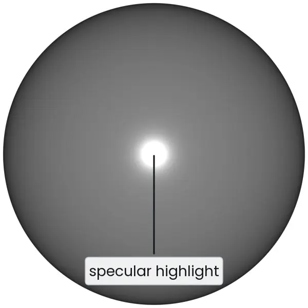
- Specular k_s·I_s·(R · V)ⁿ: the shiny highlight, strongest when the reflected ray points at the viewer; the shininess exponent n controls its size (n = 1 is a broad glow, n = 200 a tiny sharp spot).
Attenuation divides the diffuse and specular terms of a point light by a factor such as 1/(c₁ + c₂d + c₃d²), where d is the distance, so that distant lights are dimmer.
Blinn–Phong replaces R · V by N · H with the halfway vector H = (L + V)/|L + V|, which is cheaper and is the form used in most real-time systems. Several lights are summed.
Colour is handled by evaluating the equation separately for red, green and blue with the material coefficients for each channel.
Take N = (0, 0, 1), light direction L = (1, 1, 1)/√3 and viewer V = (0, 0, 1), with k_a = 0.2, k_d = 0.6, k_s = 0.5 and unit light intensities.
L = (0.5774, 0.5774, 0.5774), so N · L = 0.5774. Reflection R = 2(N · L)N − L = (-0.5774, -0.5774, 0.5774), so R · V = 0.5774. Ambient = 0.200, diffuse = 0.6 × 0.5774 = 0.3464. The specular term depends strongly on n:
| Shininess n | (R·V)ⁿ | Specular k_s·(R·V)ⁿ | Total I = ambient + diffuse + specular |
|---|---|---|---|
| 1 | 0.5774 | 0.2887 | 0.8351 |
| 10 | 0.0041 | 0.0021 | 0.5485 |
| 50 | 0.0000 | 0.0000 | 0.5464 |
| 200 | 0.0000 | 0.0000 | 0.5464 |
With n = 10 the total is 0.5485.
The viewer sits at an angle to the mirror direction (R · V = 0.5774, about 54.7°), so for large n the specular term vanishes and only the matte parts remain: highlights appear only near the mirror direction.
In Blinn–Phong the halfway vector H = (0.3251, 0.3251, 0.8881) gives N · H = 0.8881, a different but related number (the exponents are chosen differently to give a similar highlight size).
6.3 Surface shading methods
A polygon mesh approximates a smooth surface; the illumination model can be applied at different points.
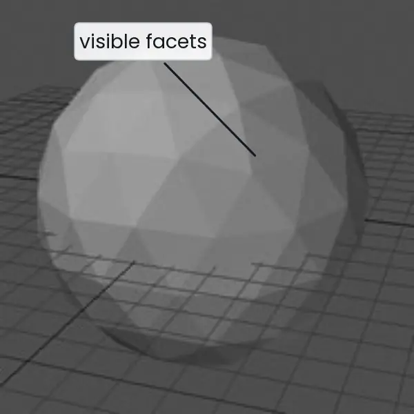
- Flat (constant) shading: compute one intensity per polygon (using its normal) and fill the whole polygon with it. It is fastest but shows visible facets, and Mach-band effects exaggerate the edges.
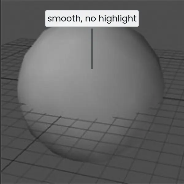
- Gouraud shading: compute the intensity at each vertex using a vertex normal (the average of the normals of the polygons sharing the vertex), then interpolate the intensity linearly along edges and across the scan line. It removes facets cheaply but can miss highlights that fall inside a polygon and cause Mach bands.
- Phong shading: interpolate the normal across the polygon and evaluate the illumination model at every pixel. It gives accurate highlights and smooth specular reflection at a higher cost (Phong shading is the interpolation method; the Phong model is the lighting equation, and they are often confused).
An edge joins two vertices with normals N₁ = (-0.60, 0.00, 0.80) and N₂ = (0.60, 0, 0.80), the light and the viewer are both along +z (L = V = (0, 0, 1)), n = 50, and the coefficients are as before.
At each vertex N · L = 0.8, but R · V = 2(0.8)² − 1 = 0.28, and 0.28⁵⁰ is practically zero, so the intensity at both ends is 0.6800 (ambient 0.2 + diffuse 0.48). Gouraud shading interpolates the intensities: the midpoint gets 0.6800.
Phong shading interpolates the normal first: the midpoint normal is (0.00, 0.00, 1.00), pointing straight at the viewer and the light, so N · L = 1, R · V = 1 and the intensity is 0.2 + 0.6 + 0.5 = 1.3000 (clamped to 1.0 on a display).
Gouraud shading shows a flat, dim edge; Phong shading shows a bright specular highlight, because the highlight lies between the vertices where Gouraud never evaluates the lighting. The Gouraud value is 47.7% below the Phong value.
| Flat | Gouraud | Phong | |
|---|---|---|---|
| Computed | Per polygon | Per vertex, intensity interpolated | Per pixel, normal interpolated |
| Cost | Lowest | Moderate | Highest |
| Facets visible | Yes | Reduced | No |
| Highlights | Poor | May be missed | Accurate |
6.4 Beyond local shading
Texture mapping wraps an image onto a surface using (u, v) coordinates stored at the vertices; bump mapping perturbs normals to imitate roughness; environment maps fake reflections.
Shadows come from shadow maps (render depth from the light) or shadow volumes. Transparency blends colours with an alpha value: C = α·C_source + (1 − α)·C_background.
Ray tracing follows rays from the eye through each pixel, finds the nearest hit and spawns shadow, reflection and refraction rays recursively, producing realistic mirrors and glass; global illumination (radiosity, path tracing) also accounts for light bouncing between surfaces.
Real-time engines combine rasterisation with ray tracing hardware.
6.5 Seeing the ideas: depth buffers, vectors, highlights and shading
Hidden-surface removal and shading are best understood by watching numbers turn into pictures.
The plate shows what the three shading methods actually look like; the figures trace the Z-buffer of section 6.1, the vectors and intensities of section 6.2, and the highlight that Gouraud shading misses in section 6.3.


6.5.1 Eight applications of hidden-surface removal and shading
- Video games. Every GPU runs a Z-buffer, so the player always sees the nearest wall, tree or character without any sorting by the programmer. Lighting is computed per pixel with a Blinn–Phong style model, so that metal and plastic look different. This is why a mobile game can draw thousands of overlapping objects smoothly.
- Architectural walkthroughs. An architect in Kathmandu can show a client a house before it is built, with walls that hide the rooms behind them and light that falls from the windows. Shading makes the flat drawing look like a real building. Clients can then judge the design before spending money on construction.
- Animated films and television advertisements. Studios use ray tracing and global illumination for realistic glass, water and skin. The shading models of this unit are the starting point and are refined with textures and shadows. Even a short advertisement shot for Nepali television relies on these steps.
- Computer-aided design (CAD). Engineers working on machine parts or a hydropower turbine need solid-looking models where hidden edges are removed. Shaded views let them see curved surfaces and check the shape. Wireframe views alone would show confusing lines through the part.
- Medical visualisation. CT and MRI data are turned into 3D images of bones and organs, where the nearest surface hides the rest and shading shows its shape. A doctor can see a fracture in depth instead of reading a stack of flat slices. This helps in planning surgery and explaining it to patients.
- Virtual reality and training simulators. A flight, driving or surgery simulator must show correct occlusion and lighting at 60 frames per second or more. The Z-buffer and simple per-pixel shading are fast enough for this. A driving-school simulator can teach road signs and mountain roads safely.
- Online product viewers. A shop can show a 3D phone, watch or shoe that the customer rotates with the mouse. The specular highlight tells the eye whether the surface is glossy or matte. Good shading makes a product look real and builds trust in a purchase made online.
- Scientific and map visualisation. Terrain models of the Himalayas use a shading called hill-shading, a diffuse term with the sun placed in the north-west, so that ridges and valleys become visible. Molecule viewers and weather models use the same hidden-surface and shading ideas. A single picture can then show thousands of measurements at once.
Chapter summary
- The Z-buffer keeps the nearest depth per pixel and works for any surface; painter's algorithm sorts and overwrites; back-face culling removes rear faces.
- The Phong model is ambient + diffuse (N · L) + specular (R · V)ⁿ; Blinn–Phong uses N · H.
- Flat shading uses one intensity per polygon, Gouraud interpolates vertex intensities, Phong interpolates normals and lights every pixel.
- Gouraud shading can miss a highlight inside a polygon; Phong shading captures it.
- Textures, shadow maps, alpha blending and ray tracing add realism.
Practice
- Describe the Z-buffer algorithm and state its main memory cost for 1280 × 720 with 32-bit depth.
- Why does the painter's algorithm fail for cyclically overlapping polygons?
- Write the three terms of the Phong model and say what each represents.
- Compute N · L for N = (0, 1, 0) and L = (0.6, 0.8, 0).
- Compute the diffuse term for k_d = 0.5, I_d = 1 and N · L = 0.8.
- What is the effect of increasing the shininess exponent n?
- Differentiate Gouraud and Phong shading.
- What is the halfway vector in Blinn–Phong?
- Compute the colour blend with α = 0.25, source = 200 and background = 40.
- How does ray tracing produce shadows?
Answers and worked solutions
1. For each polygon pixel compare its depth with the stored depth and, if nearer, update colour and depth. Memory: 1280 × 720 × 4 bytes = 36,86,400 bytes (3.5 MiB).
2. There is no consistent far-to-near order when polygons overlap in a cycle (A over B over C over A), so any painting order shows an error unless a polygon is split.
3. Ambient (constant background light), diffuse (matte reflection proportional to N · L), specular (shiny highlight proportional to (R · V)ⁿ).
4. 0 × 0.6 + 1 × 0.8 + 0 × 0 = 0.8.
5. 0.5 × 1 × 0.8 = 0.40.
6. The highlight becomes smaller and sharper (shinier surface).
7. Gouraud interpolates intensities computed at vertices; Phong interpolates normals and evaluates the lighting at each pixel.
8. H = (L + V)/|L + V|, the direction halfway between the light and the viewer; N · H replaces R · V.
9. 0.25 × 200 + 0.75 × 40 = 50 + 30 = 80.
10. It casts a ray from the surface point towards the light; if the ray hits an object first, the point is in shadow and the light's contribution is omitted.
Model answers: medium (5 marks) and long (10 marks) questions
Q1 (5 marks). Explain the Z-buffer (depth-buffer) algorithm. Trace it for a 3 × 3 screen with polygon P (depth 6 at pixels x, y in {0, 1}), polygon Q (depth 4 at x, y in {1, 2}) and polygon R (depth 3, 5 and 7 at x = 0, 1, 2 of row y = 2).
Introduction. The Z-buffer is an image-space hidden-surface method that stores, for every pixel, the depth of the nearest surface drawn so far (section 6.1, Figure 6.1).
- Initialise. Set every depth to infinity and every colour to the background.
- For each polygon, for each covered pixel find the depth z.
- Compare. If z is smaller than the stored depth, store z and the polygon's colour; otherwise discard the pixel.
- Result. After all polygons the frame buffer shows the nearest surface at each pixel, in any drawing order.
Trace. Each pixel is written as depth/polygon, with “–” for nothing drawn.
| x = 0 | x = 1 | x = 2 | |
|---|---|---|---|
| y = 0 | 6 / P | 6 / P | – |
| y = 1 | 6 / P | 4 / Q | 4 / Q |
| y = 2 | 3 / R | 4 / Q | 4 / Q |
P covers 4 pixels, Q covers 4 and R covers 3, so 11 depth tests are made. Q beats P at (1, 1) since 4 < 6. R is drawn at (0, 2) because that pixel was empty (3 < infinity), but loses at (1, 2) (5 > 4) and at (2, 2) (7 > 4).
Drawing in the order R, Q, P gives exactly the same table.
Conclusion. The Z-buffer needs no sorting and handles intersecting surfaces, but uses memory: a 1920 × 1080 buffer of 32-bit depths needs 8,294,400 bytes (7.9 MiB).
Q2 (5 marks). State the Phong illumination model. Find the intensity at a point with N = (0, 0, 1), L = (0, 0.6, 0.8), V = (0, 0, 1), k_a = 0.1, k_d = 0.5, k_s = 0.4 and unit light intensities, for n = 1, 5 and 20.
Introduction. The Phong model gives the intensity of light leaving a surface point towards the viewer as the sum of ambient, diffuse and specular parts (section 6.2, Figure 6.3): I = k_a I_a + k_d I_d (N · L) + k_s I_s (R · V)ⁿ, with R = 2(N · L)N − L.
Calculation. N · L = 0.8, so the diffuse part is 0.5 × 0.8 = 0.400. R = 2(0.8)(0, 0, 1) − (0, 0.6, 0.8) = (0, −0.6, 0.8), and R · V = 0.8. The ambient part is 0.100.
| n | (R · V)ⁿ | Specular 0.4 (R · V)ⁿ | Total I |
|---|---|---|---|
| 1 | 0.8000 | 0.3200 | 0.8200 |
| 5 | 0.3277 | 0.1311 | 0.6311 |
| 20 | 0.0115 | 0.0046 | 0.5046 |
| 100 | 0.0000 | 0.0000 | 0.5000 |
Observation. Ambient and diffuse parts (0.500 together) do not depend on n. Only the specular part falls as n rises, so a large n gives a small, sharp highlight.
With the Blinn–Phong halfway vector H = (0, 0.316, 0.949), N · H = 0.949 and (N · H)²⁰ = 0.349, giving a total of 0.639.
Conclusion. The Phong model is cheap and gives believable matte and shiny materials, but it is empirical and ignores light bouncing between surfaces.
Q3 (5 marks). Differentiate flat, Gouraud and Phong shading. Why does Gouraud shading miss a highlight that lies between two vertices?
Introduction. A polygon mesh only approximates a smooth surface, so the lighting equation can be applied at different places (section 6.3, Figure 6.5 and Plate 6.1).
- Flat shading computes one intensity per polygon using its normal. It is fastest but the facets are visible.
- Gouraud shading computes intensity at each vertex with an averaged vertex normal and interpolates the intensity across the polygon. Facets are hidden at moderate cost.
- Phong shading interpolates the normal across the polygon and evaluates the lighting equation at every pixel. It is the most accurate and the most expensive.
Missed highlight. Take an edge with end normals (−0.6, 0, 0.8) and (0.6, 0, 0.8), light and viewer along +z, n = 50, k_a = 0.2, k_d = 0.6, k_s = 0.5.
At both ends N · L = 0.8 and R · V = 2(0.8)² − 1 = 0.28, and 0.28⁵⁰ is almost zero, so the intensity is 0.2 + 0.48 = 0.68. Gouraud shading interpolates 0.68 and 0.68, so the midpoint also gets 0.68.
Phong shading interpolates the normal first: the midpoint normal is (0, 0, 1), N · L = R · V = 1, and I = 0.2 + 0.6 + 0.5 = 1.30.
The highlight occurs only between the vertices, where Gouraud shading never evaluates the lighting; its value is 47.7% below the Phong value.
Conclusion. Phong shading is needed for shiny surfaces, while Gouraud shading is adequate for matte ones.
Q4 (10 marks). Describe the hidden-surface removal methods used in computer graphics and compare them.
Introduction. When a 3D scene is projected, several surfaces may fall on the same pixel, and only the nearest should be shown. Hidden-surface removal (visible-surface determination) decides which one.
The methods are either object-space (compare objects with each other) or image-space (decide pixel by pixel) (section 6.1, Figures 6.1 and 6.2).
- Back-face culling. Faces whose normal satisfies N · V ≤ 0 point away from the viewer and are discarded. It removes about half of the polygons of a closed solid, but cannot order overlapping front faces, so it is only a first step.
- Depth (Z) buffer. A depth value per pixel is compared with each new polygon's depth, keeping the nearer. It is simple, needs no sorting and handles intersecting surfaces. Its cost is memory (7.9 MiB for a 1920 × 1080 buffer of 32-bit depths) and z-fighting for nearly coplanar surfaces.
- Painter's algorithm (depth sort). Polygons are sorted far to near and painted in that order. It needs sorting every frame and fails for cyclic overlap and for intersecting polygons, which must be split.
- Scan-line method. For each scan line, the visible polygon in each span between edge crossings is found, using depth only where polygons overlap. It uses coherence along the line.
- Area subdivision (Warnock). The window is split recursively until each piece contains at most one visible surface or is one pixel.
- BSP trees. A binary space partition fixes a correct far-to-near order for a static scene, which can then be reused from any viewpoint.
- Ray casting. A ray from the eye through each pixel is intersected with the objects and the nearest hit is taken; this is the basis of ray tracing.
- A-buffer. An extension of the Z-buffer that keeps a list of surfaces per pixel, so transparency and anti-aliasing can be handled.
| Method | Space | Sorting | Handles intersections | Typical use |
|---|---|---|---|---|
| Back-face | Object | None | n/a (partial) | First step for solids |
| Z-buffer | Image | None | Yes | All GPUs |
| Painter's | Object | Yes | No (split) | Simple 2.5D scenes |
| Scan-line | Image | Partial | Yes | Software renderers |
| Area subdivision | Image | None | Yes | Teaching, research |
| BSP tree | Object | Precomputed | By splitting | Static game levels |
| Ray casting | Image | None | Yes | Ray tracing |
Conclusion. The Z-buffer wins in practice because it is simple, independent of the number of polygons and implemented in hardware. Back-face culling is used before it to save work, and ray casting extends to ray tracing for realistic effects.
Q5 (10 marks). Explain illumination models and surface shading methods in computer graphics, with the Phong model and a comparison of flat, Gouraud and Phong shading.
Introduction. Once the visible surface of a pixel is known, its colour must be computed.
An illumination model gives the light leaving a surface point towards the viewer; a shading method decides where on a polygon mesh the model is evaluated (sections 6.2 and 6.3, Figures 6.3 to 6.5 and Plate 6.1).
- Ambient term. k_a I_a is a constant that stands for light scattered everywhere, so shadowed faces are not black.
- Diffuse term. k_d I_d (N · L) is Lambert's law: matte reflection, brightest when the surface faces the light and independent of the viewer.
- Specular term. k_s I_s (R · V)ⁿ is the shiny highlight with R = 2(N · L)N − L; the exponent n sets its size (a larger n gives a smaller spot).
- Attenuation and several lights. Light intensity falls as 1/(c₁ + c₂d + c₃d²) with distance d and the contributions of all lights are added; the equation is evaluated separately for red, green and blue.
- Blinn–Phong. Replacing R · V by N · H, with H = (L + V)/|L + V|, is cheaper and is used in most real-time systems.
- Flat shading. One intensity per polygon; the fastest method, but facets and Mach bands show.
- Gouraud shading. Intensity is computed at vertices (with averaged normals) and interpolated; smooth and cheap but may miss highlights inside polygons.
- Phong shading. The normal is interpolated and the model is evaluated at every pixel, giving accurate highlights at the highest cost.
Worked example. For N = (0, 0, 1), L = (0, 0.6, 0.8), V = (0, 0, 1), k_a = 0.1, k_d = 0.5, k_s = 0.4 and n = 20, I = 0.1 + 0.4 + 0.4 × 0.8²⁰ = 0.1 + 0.4 + 0.0046 = 0.5046.
For an edge with end normals (±0.6, 0, 0.8), Gouraud shading gives 0.68 at the midpoint while Phong shading gives 1.30.
| Flat | Gouraud | Phong | |
|---|---|---|---|
| Evaluated | Per polygon | Per vertex | Per pixel |
| Interpolated | Nothing | Intensity | Normal |
| Facets visible | Yes | Reduced | No |
| Highlights | Poor | May be missed | Accurate |
| Cost | Lowest | Moderate | Highest |
Conclusion. The Phong illumination model is the common local model, and the choice of shading method trades cost against realism. For effects such as shadows and mirrors, textures, shadow maps or ray tracing are added.