Time, Clocks and Global State

Two servers log "payment received at 10:00:00.120" and "order created at 10:00:00.095". Which happened first? If their clocks differ by 50 ms the logs cannot tell you.

Time is the first thing a single computer gives you for free and a distributed system cannot: every machine has its own oscillator, and messages take unpredictable time.

This unit shows how to synchronise physical clocks (Cristian, Berkeley, NTP) and, more importantly, how to avoid needing them by using logical clocks (Lamport, vector) that capture only the order that matters, namely causality.

3.1 Physical clocks, drift and skew

A computer clock counts the ticks of a quartz crystal. Crystals run slightly fast or slow, by a drift rate ρ often quoted in parts per million (ppm). A typical commodity clock has ρ around 10 ppm.

Skew is the difference between two clocks at one instant; offset is the difference from a reference.

rho = 10e-6
print(f"drift per day: {rho * 86400:.3f} s")
print(f"resync interval for 1 ms skew: {0.001 / (2 * rho):.0f} s")

drift per day: 0.864 s
resync interval for 1 ms skew: 50 s

A 10 ppm clock gains or loses 0.864 s per day. Two clocks drifting in opposite directions diverge at up to 2ρ, so to keep them within δ of each other they must resynchronise at least every δ / 2ρ, which is 50 s for δ = 1 ms.

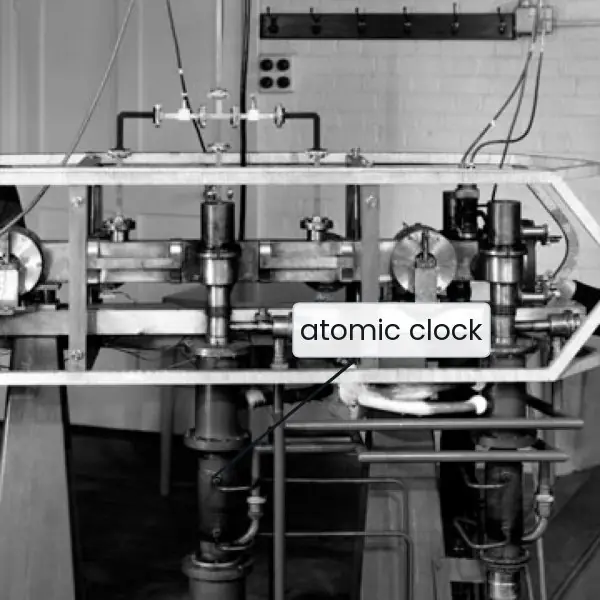
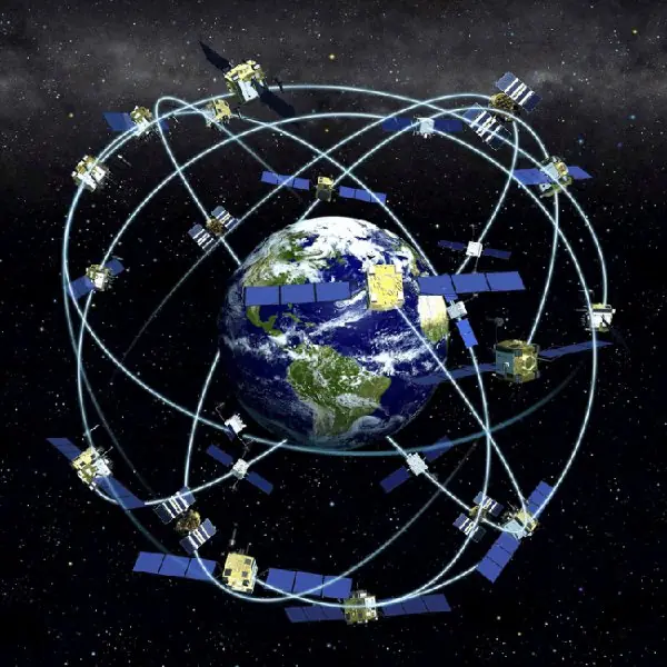
Reference time comes from UTC, distributed by radio time signals, GPS satellites (atomic clocks, accuracy tens of nanoseconds) and, over the internet, by NTP.

Never set a clock backwards abruptly: programs measuring durations would see negative time. Good implementations slew (run slightly faster or slower) until the error is gone, and measure intervals with a monotonic clock.

3.2 Cristian's algorithm

A client asks a time server (with a UTC receiver) for the time. Let T₀ be the client's clock when it sends the request and T₁ when the reply arrives; the server reports Tₛ. The reply spent unknown time in transit, so the client assumes it was half the round trip:

estimate of server time at receipt = Tₛ + (T₁ − T₀) / 2, and the client sets its clock to this (or slews towards it).

If the minimum one-way delay is min, the true server time lies between Tₛ + min and Tₛ + RTT − min, so the accuracy is ± (RTT/2 − min). A small RTT means a better estimate, so clients send several requests and keep the one with the smallest round trip.

samples = [(1000, 1040, 1520), (2000, 2016, 2490), (3000, 3100, 3560)]
best = None
for T0, T1, Ts in samples:
    rtt = T1 - T0
    est = Ts + rtt / 2
    print(f"RTT={rtt:3d} ms  estimated server time={est:7.1f}  offset to apply={est - T1:+7.1f} ms")
    if best is None or rtt < best[0]:
        best = (rtt, est - T1)
min_one_way = 5
print(f"best sample RTT={best[0]} ms: offset {best[1]:+.1f} ms, error bound +/- {best[0] / 2 - min_one_way:.1f} ms")

RTT= 40 ms  estimated server time= 1540.0  offset to apply= +500.0 ms
RTT= 16 ms  estimated server time= 2498.0  offset to apply= +482.0 ms
RTT=100 ms  estimated server time= 3610.0  offset to apply= +510.0 ms
best sample RTT=16 ms: offset +482.0 ms, error bound +/- 3.0 ms

The three samples give offsets of +500, +482 and +510 ms: the third, with RTT 100 ms, is least trustworthy. The best sample has RTT 16 ms and a guaranteed error of at most ±3.0 ms when the minimum one-way delay is 5 ms.

Weaknesses: a single time server is a single point of failure and a target for a fake server; there is no defence against a malicious or faulty server.

3.3 The Berkeley algorithm

Berkeley UNIX's time daemon needs no UTC source.

A master polls all machines for their clock values, estimates each machine's clock difference using round-trip times, takes the average (ignoring clocks that differ by more than a threshold, which are probably faulty), and tells each machine how much to adjust, not the new absolute time, since the adjustment is robust to message delay.

The classic example: master 3:00, slaves 2:50 and 3:25.

clocks = {"master": 180, "s1": 170, "s2": 205}
def berkeley(clocks, limit=None):
    m = clocks["master"]
    diffs = {k: v - m for k, v in clocks.items()}
    used = {k: d for k, d in diffs.items() if limit is None or abs(d) <= limit}
    avg = sum(used.values()) / len(used)
    return avg, {k: (m + avg) - v for k, v in clocks.items()}

for limit in (None, 20):
    avg, adj = berkeley(clocks, limit)
    print(f"limit={limit}: average offset {avg:+.1f} min, adjustments {adj}")

limit=None: average offset +5.0 min, adjustments {'master': 5.0, 's1': 15.0, 's2': -20.0}
limit=20: average offset -5.0 min, adjustments {'master': -5.0, 's1': 5.0, 's2': -30.0}

Clock values are minutes since noon. With no limit the differences are 0, −10 and +25, average +5, so the master advances 5 minutes, slave 1 advances 15 and slave 2 goes back 20 (in practice by slowing the clock).

With a 20-minute fault threshold slave 2's value is ignored: the average of the master and slave 1 is −5, and slave 2 is still told to correct by −30 minutes to rejoin the group.

Berkeley gives internal consistency (the group agrees) rather than agreement with true time.

3.4 The Network Time Protocol

NTP synchronises clients to UTC over the internet through a hierarchy of strata (stratum 0 = reference clocks, stratum 1 = servers attached to them, stratum 2 = clients of stratum 1, and so on).

One exchange records four timestamps: t₀ client send, t₁ server receive, t₂ server send, t₃ client receive.

• offset θ = ((t₁ − t₀) + (t₂ − t₃)) / 2
• round-trip delay δ = (t₃ − t₀) − (t₂ − t₁)

t0, t1, t2, t3 = 1000, 1060, 1062, 1026
theta = ((t1 - t0) + (t2 - t3)) / 2
delta = (t3 - t0) - (t2 - t1)
print(f"offset theta = {theta} ms, round-trip delay delta = {delta} ms")
print(f"true offset 50 ms; error = {theta - 50} ms = (up - down)/2 with up=10, down=14")

offset theta = 48.0 ms, round-trip delay delta = 24 ms
true offset 50 ms; error = -2.0 ms = (up - down)/2 with up=10, down=14

The calculation cancels the server's processing time (t₂ − t₁) from the delay. The remaining error equals half the difference between outbound and return delays, here (10 − 14)/2 = −2 ms.

NTP can never remove path asymmetry; it filters eight recent samples, keeps the lowest-delay one and combines several servers to reject bad ones. On a LAN it achieves about a millisecond; across the internet, tens of milliseconds.

PTP (IEEE 1588) with hardware timestamping reaches microseconds in data centres. Google's TrueTime exposes clock uncertainty as an interval and makes transactions wait out the uncertainty to order commits globally (Spanner).

3.5 Happened-before and Lamport clocks

Lamport (1978) observed that we need not agree on the time, only on the order of events that could affect each other. The happened-before relation → is the smallest relation such that:

1. If a and b are in the same process and a occurs before b, then a → b.
2. If a is the sending of a message and b is its receipt, then a → b.
3. If a → b and b → c, then a → c (transitivity).

Events with neither a → b nor b → a are concurrent (a ∥ b); they cannot have influenced each other. A Lamport logical clock is an integer counter per process:

1. Before each event, a process increments its clock: Lᵢ = Lᵢ + 1.
2. A message carries the sender's timestamp t.
3. On receipt, the receiver sets Lⱼ = max(Lⱼ, t) + 1.

This guarantees the clock condition: a → b implies L(a) < L(b). The converse is false: L(a) < L(b) does not imply a → b. To get a total order consistent with causality, break ties by process ID: sort by (L, pid).

Total ordering is the foundation of Ricart–Agrawala mutual exclusion (Unit 4) and replicated state machines.

3.6 Vector clocks

To detect concurrency, each process keeps a vector V of N counters.

Rules: on any local or send event, Vᵢ[i] = Vᵢ[i] + 1 (a send carries the vector); on receipt of vector W, set Vᵢ[k] = max(Vᵢ[k], W[k]) for all k, then Vᵢ[i] = Vᵢ[i] + 1.

Compare vectors componentwise: V(a) < V(b) if every component of V(a) is ≤ that of V(b) and the vectors differ; then a → b. If neither vector is ≤ the other, the events are concurrent.

The next program runs both clocks on a nine-event, three-process execution and lists the concurrent pairs.

procs = ["P1", "P2", "P3"]
events = [("P1", "local", None), ("P1", "send", "m1"), ("P2", "local", None),
          ("P2", "recv", "m1"), ("P3", "local", None), ("P2", "send", "m2"),
          ("P3", "recv", "m2"), ("P3", "send", "m3"), ("P1", "recv", "m3")]
L = {p: 0 for p in procs}
V = {p: [0, 0, 0] for p in procs}
inflight, rows = {}, []
for n, (p, kind, m) in enumerate(events, 1):
    i = procs.index(p)
    if kind == "recv":
        L[p] = max(L[p], inflight[m][0]) + 1
        V[p] = [max(x, y) for x, y in zip(V[p], inflight[m][1])]
        V[p][i] += 1
    else:
        L[p] += 1
        V[p][i] += 1
        if kind == "send":
            inflight[m] = (L[p], list(V[p]))
    rows.append((n, p, kind, m or "-", L[p], tuple(V[p])))
for r in rows:
    print("e%d  %s %-5s %-2s  L=%d  V=%s" % r)

def before(u, v):
    return all(x <= y for x, y in zip(u, v)) and u != v

vec = {r[0]: r[5] for r in rows}
pairs = [(a, b) for a in vec for b in vec if a < b
         and not before(vec[a], vec[b]) and not before(vec[b], vec[a])]
print("concurrent pairs:", pairs)

e1  P1 local -   L=1  V=(1, 0, 0)
e2  P1 send  m1  L=2  V=(2, 0, 0)
e3  P2 local -   L=1  V=(0, 1, 0)
e4  P2 recv  m1  L=3  V=(2, 2, 0)
e5  P3 local -   L=1  V=(0, 0, 1)
e6  P2 send  m2  L=4  V=(2, 3, 0)
e7  P3 recv  m2  L=5  V=(2, 3, 2)
e8  P3 send  m3  L=6  V=(2, 3, 3)
e9  P1 recv  m3  L=7  V=(3, 3, 3)
concurrent pairs: [(1, 3), (1, 5), (2, 3), (2, 5), (3, 5), (4, 5), (5, 6)]

Study the trace. Event e4 (P2 receives m1) has L = 3 and V = (2, 2, 0): it knows two events at P1 and its own two.

Event e5 at P3 has L = 1 while e4 has L = 3, yet V(e5) = (0, 0, 1) and V(e4) = (2, 2, 0) are incomparable, so the events are concurrent.

The Lamport number alone would suggest e5 came "earlier"; only the vector reveals that there is no causal path. The price is a vector of N integers on every message.

Uses. Dynamo-style stores attach vector clocks to object versions to detect conflicting concurrent writes (siblings) that the application must merge; causal ordering of messages (deliver a message only after everything that causally precedes it) uses vectors; version-control systems and CRDTs rely on the same idea.

Hybrid logical clocks combine a physical timestamp with a logical counter to stay close to wall-clock time while keeping causality.

3.7 Seeing time: clocks, clock servers and event diagrams

Time in a distributed system comes from physical devices and from counting events. Plate 3.1 shows three physical sources of time and of the people who reasoned about it, and Figures 3.1 to 3.3 show the algorithms that turn them into agreement.

(a) First caesium clock, 1955

(b) Leslie Lamport

(c) GPS constellation

3.7.1 Eight uses of synchronised and logical time

1. Ordering log records. When many servers write logs, an engineer must know which event came first. Wall-clock stamps from synchronised servers allow a rough order, and logical clocks give a safe one. This is how the cause of a failed payment is traced across several services.
2. Certificate and token validity. A website certificate or a login token is valid between two dates and times. A device whose clock is wrong by a day may reject a good certificate or accept an expired one. This is why phones and servers run NTP all the time.
3. Expiry of leases and sessions. A lock lease or a login session ends after a set time. The holder and the server must agree closely on how long a second is. Clock drift of 50 ppm adds up to 4.32 seconds a day if it is never corrected.
4. Fair ordering of transactions. A bank, a stock exchange or a ticket system must decide who was first. Timestamps with a tie-break on the node identifier give every event a unique place in a total order. Two payments to the same account are then always applied in the same order on every replica.
5. Detecting conflicting updates. Vector clocks show whether one version of a record comes after another or whether they are concurrent. Systems such as Amazon's Dynamo use them to keep both concurrent versions and ask the application to merge them. This avoids silently losing a student's edit made on an offline phone.
6. Consistent snapshots and backups. To record a global state of many processes, we must pick a cut that respects the order of messages. Logical time tells us which cuts are consistent. Backup and debugging tools use this to restore a system to a state that could really have happened.
7. Cellular and radio networks. Mobile base stations must transmit in exact time slots, so they take time from GPS or from a network clock. A drift of a few microseconds would make neighbouring stations interfere. Nepali operators and the broadcasters rely on the same source of precise time.
8. Scientific and financial records. Experiments such as the CERN grid in Plate 1.1 stamp every measurement with a precise time so that data from many sites can be joined. In finance, regulations require records stamped within a small error of UTC. Synchronised clocks make such audits possible.

Chapter summary

• Physical clocks drift at ρ (about 10 ppm = 0.864 s/day); synchronisation must repeat about every δ/2ρ.
• Cristian: estimate = Tₛ + RTT/2, accuracy ± (RTT/2 − min). Berkeley: average clock differences and send each node its adjustment. NTP: θ = ((t₁−t₀)+(t₂−t₃))/2, δ = (t₃−t₀) − (t₂−t₁); path asymmetry remains as error.
• Happened-before is a partial order; Lamport clocks give L(a) < L(b) whenever a → b but not the converse; vector clocks give a → b ⇔ V(a) < V(b) and expose concurrency.

Practice

1. Differentiate clock drift, skew and offset.
2. A clock drifts at 20 ppm. How much error accumulates in one day? How often must it be corrected to stay within 5 ms of a perfect clock?
3. A client sends a request at T₀ = 5,000 ms, receives the reply at T₁ = 5,030 ms, and the server timestamp is 5,400 ms. Find the client's estimate of the server time and the offset. If the minimum one-way delay is 8 ms, what is the error bound?
4. Three clocks read 10:00, 10:06 and 9:57 (minutes). The master (10:00) runs Berkeley without a fault threshold. Give each node's adjustment.
5. NTP timestamps: t₀ = 200, t₁ = 330, t₂ = 332, t₃ = 242 (ms). Compute θ and δ.
6. State the Lamport clock rules. If L(a) < L(b) , can we conclude a → b?
7. Vectors: A = (3, 1, 0), B = (2, 2, 1), C = (3, 2, 1). Classify each pair as before, after or concurrent.
8. Why can't Lamport clocks detect concurrent events but vector clocks can? What is the cost?
9. Why should a program never measure a duration by subtracting two wall-clock readings?

Answers and worked solutions

1. Drift: the rate at which a clock gains or loses time. Skew: difference between two clocks at one instant. Offset: difference between a clock and a reference.

2. 20 × 10⁻⁶ × 86,400 = 1.728 s per day. Within 5 ms of a perfect clock: 0.005 / 20×10⁻⁶ = 250 s.

3. RTT = 30 ms; estimate = 5,400 + 15 = 5,415 ms; offset = 5,415 − 5,030 = +385 ms; bound = 15 − 8 = ±7 ms.

4. Differences from master: 0, +6, −3; average = +1 minute. Adjustments: master +1, second clock 1 − 6 = −5, third +1 + 3 = +4 minutes (all set to 10:01).

5. θ = ((330 − 200) + (332 − 242)) / 2 = (130 + 90)/2 = 110 ms; δ = (242 − 200) − (332 − 330) = 42 − 2 = 40 ms.

6. Increment before each event; messages carry the timestamp; on receipt L = max(L, t) + 1. No: L(a) < L(b) is also possible for concurrent events.

7. A vs B: A₁ = 3 > 2 but A₂ = 1 < 2, so concurrent. A vs C: (3,1,0) ≤ (3,2,1), so A before C. B vs C: (2,2,1) ≤ (3,2,1), so B before C.

8. A Lamport clock is one integer, so two incomparable histories can still be ordered numerically. A vector holds per-process counts, so incomparability is visible. Cost: N integers per message and per version.

9. The wall clock may be stepped by NTP or a manual change and can go backwards; use a monotonic clock for durations.

Model answers: medium (5 marks) and long (10 marks) questions

Q1 (5 marks). Explain Cristian's and the Berkeley algorithms. Compute one example of each.

Introduction. Both algorithms synchronise physical clocks over a network whose delay is not known exactly (sections 3.2 and 3.3, Figures 3.1 and 3.2).

1. Cristian: idea. A client asks a time server that has a UTC source. It measures the round trip RTT = T1 - T0 and assumes the reply took half of it.
2. Cristian: example. With T0 = 0 ms, T1 = 40 ms and Ts = 5020 ms, RTT = 40 ms and the new time is 5020 + 20 = 5040 ms. If the minimum one-way delay is 5 ms, the accuracy is +/- (20 - 5) = +/- 15 ms.
3. Berkeley: idea. No machine has UTC. The master polls all machines, computes the average difference and tells each machine how much to adjust, so message delay matters less.
4. Berkeley: example. Clocks 3:00 (master), 2:50 and 3:25 differ from the master by 0, -10 and +25 minutes. The average is +5 minutes, so the common time is 3:05 and the adjustments are +5, +15 and -20 minutes.
5. Practice. Clocks are slewed (run slightly faster or slower) so that time never goes backwards. Real systems use NTP, which adds filtering and a hierarchy of strata.

Feature	Cristian	Berkeley
Time source	external UTC server	none, internal average
Who computes	client	master
Messages	2 per client	polling plus adjustments
Accuracy	+/- RTT/2	agreement only

Conclusion. Use Cristian when a reliable time server exists and Berkeley when only mutual agreement is needed.

Q2 (5 marks). State the happened-before relation and the rules of Lamport logical clocks. Timestamp the events of the diagram in Figure 3.3.

Introduction. Without a global clock we cannot compare physical times, so Lamport (1978) defined an ordering based only on events and messages (section 3.5).

1. Happened-before. a to b holds if a and b are in the same process and a comes first, or a sends a message that b receives, or by transitivity. Events not related by it are concurrent.
2. Rule 1. Before each local or send event, a process increments its counter: C = C + 1.
3. Rule 2. A message carries the sender's counter. On receipt, the receiver sets C = max(C, message counter) + 1.
4. Result. If a to b, then C(a) < C(b) . The converse is false.
5. Application to the diagram. The program gives the following timestamps.

Event	Process	Kind	Lamport
a	P1	local	1
b	P1	send m1	2
c	P2	recv m1	3
d	P2	send m2	4
e	P3	local	1
f	P3	recv m2	5
g	P3	send m3	6
h	P1	recv m3	7

Conclusion. Lamport clocks give a consistent total order (ties broken by process id) but cannot show that two events are concurrent; vector clocks can.

Q3 (10 marks). Explain why physical clocks are not enough in a distributed system, describe vector clocks with an example, and compare them with Lamport clocks.

Introduction. Every computer has its own quartz clock, and no two run at exactly the same rate. A typical drift of 50 ppm is 4.32 seconds a day.

To keep two clocks within 10 ms of each other the system must resynchronise at least every 100 seconds. Even then message delay varies, so wall-clock time cannot decide the order of close events.

Physical synchronisation. GPS and atomic clocks give UTC; Cristian's algorithm and NTP copy it across the network with an error of about half the round trip (Figure 3.1); the Berkeley algorithm averages the clocks of a group (Figure 3.2).

Logical time. Lamport clocks count events, and each message carries the counter, so that a send is always stamped lower than its receive.

Vector clocks. Each process keeps a vector with one counter per process. A local or send event increments the own entry; a receive takes the entry-wise maximum with the message vector and then increments the own entry.

Vector V is before W if every entry of V is at most that of W and the vectors differ; otherwise, if neither is before the other, the events are concurrent. In Figure 3.3 the program gives the table below.

Event	Process	Kind	Lamport	Vector
a	P1	local	1	(1,0,0)
b	P1	send m1	2	(2,0,0)
c	P2	recv m1	3	(2,1,0)
d	P2	send m2	4	(2,2,0)
e	P3	local	1	(0,0,1)
f	P3	recv m2	5	(2,2,2)
g	P3	send m3	6	(2,2,3)
h	P1	recv m3	7	(3,2,3)

For example b is before h because (2,0,0) is below (3,2,3) entry by entry, while a and e are concurrent because (1,0,0) and (0,0,1) cannot be ordered. Concurrent pairs here are a||e, b||e, c||e, d||e.

Property	Lamport clock	Vector clock
Size	one integer	one integer per process
If a before b then	C(a) < C(b)	V(a) < V(b)
If C(a) < C(b) then	cannot tell	a before b only if V(a) < V(b)
Detects concurrency	no	yes
Use	total order, mutual exclusion	conflict detection in replicas

Conclusion. Physical clocks give approximate real time; logical clocks give a correct order. Vector clocks cost more space but are the tool for detecting concurrent updates.