Unit 2 · 6 teaching hours · 17 min read
Descriptive Statistics
What the syllabus asks for 4
- Measures of central tendency
- Measures of dispersion
- Pictures of centre and spread
- Eight uses of averages and measures of spread
Descriptive statistics condenses a mass of numbers into a few summary values. We need two kinds: a central value that says where the data sit, and a measure of dispersion that says how widely they spread. All values here were recomputed by bca/tools/check_stats.py.
- Mean, median, partition values (quartiles, deciles, percentiles) and mode, for raw and grouped data.
- Range, quartile deviation, mean deviation, standard deviation, variance, coefficient of variation.
- Interpretation and choice of measure.
2.1 Measures of central tendency
Arithmetic mean: \bar{x} = \frac{\sum x}{n}. For a frequency table, \bar{x} = \frac{\sum f x}{\sum f} (with x the class midpoint).
Properties: uses all values; the sum of deviations from the mean is zero \left( \sum (x - \bar{x}) = 0 \right); the sum of squared deviations is least about the mean; sensitive to outliers.
Median: the middle value of the ordered data; for n values it is the ((n + 1)/2)th item (average the two middle ones if n is even). Not affected by extreme values.
For grouped data: Median = L + ( ( \frac{n}{2} − cf)/f) × h, where L is the lower limit of the median class (the class containing the n/2th item), cf the cumulative frequency before it, f its frequency and h the class width.
Mode: the most frequent value. For grouped data: Mode = L + \left( \frac{d_{1}}{(d_{1} + d_{2})} \right) \times h, with L the lower limit of the modal class, d_{1} = f - f_{p} \mathrm{revious} ,\ d_{2} = f - f_{n} \mathrm{ext}.
A distribution may be unimodal, bimodal or have no mode. Empirical relation for moderately skewed data: mean − mode ≈ 3 ( \mathrm{mean} − median).
Partition values divide the ordered data: quartiles Q_{1} ,\ Q_{2} (= median), Q_{3} into 4 parts; deciles D_{1} \ldots D_{9} into 10; percentiles P_{1} \ldots P_{99} into 100.
Position of Q_{i} = \frac{i (n + 1)}{4} for raw data; for grouped data Q_{i} = L + ((i·n/4 − cf)/f) × h.
Marks of 10 students: 45, 52, 58, 61, 61, 67, 70, 74, 80, 92.
Mean = 660/10 = 66. Median: n = 10, the 5th and 6th values are 61 and 67, so median = 64. Mode = 61. Q_{1}: position \frac{n + 1}{4} = 2.75, between 52 and 58: 52 + 0.75 \times 6 = 56.5. Q_{3}: position 8.25, between 74 and 80: 74 + 0.25 \times 6 = 75.5.
| Class | 10–20 | 20–30 | 30–40 | 40–50 | 50–60 |
|---|---|---|---|---|---|
| Frequency f | 5 | 8 | 15 | 16 | 6 |
| Midpoint x | 15 | 25 | 35 | 45 | 55 |
| Cumulative f | 5 | 13 | 28 | 44 | 50 |
n = 50. Mean = \frac{\sum f x}{n} = \frac{75 + 200 + 525 + 720 + 330}{50} = 1850/50 = 37.
Median: \frac{n}{2} = 25 lies in the class 30–40 (cumulative 28): L = 30, cf = 13 ,\ f = 15 ,\ h = 10 \to 30 + \frac{25 - 13}{15} \times 10 = 38.
Mode: modal class 40–50 (f = 16): d_{1} = 16 - 15 = 1 ,\ d_{2} = 16 - 6 = 10 \to 40 + \frac{1}{11} \times 10 = 40.91.
Q_{1}: \frac{n}{4} = 12.5 in 20–30: 20 + \frac{12.5 - 5}{8} \times 10 = 29.375. Q_{3}: \frac{3 n}{4} = 37.5 in 40–50: 40 + \frac{37.5 - 28}{16} \times 10 = 45.94.
Which average? Mean for symmetric quantitative data and further calculation; median for skewed data or with outliers (incomes, house prices); mode for the most typical or for nominal data (the most common shoe size).
For positively skewed data mean > median > mode; negatively skewed the reverse; symmetric, all equal.
2.2 Measures of dispersion
| Measure | Formula | Notes |
|---|---|---|
| Range | max − min | crude; depends on extremes. Coefficient = (max − min)/(max + min) |
| Quartile deviation | Q D = \frac{(Q_{3} - Q_{1})}{2} | uses the middle 50%; coefficient = \frac{(Q_{3} - Q_{1})}{(Q_{3} + Q_{1})} |
| Mean deviation | M D = \sum | x - \bar{x} |
| Variance | \sigma^{2} = \frac{\sum (x - \bar{x})^{2}}{n} (population); s^{2} = \frac{\sum (x - \bar{x})^{2}}{n - 1} (sample) | squared units |
| Standard deviation | \sigma = \sqrt{\sigma^{2}} | same units as data; most used |
| Coefficient of variation | C V = \left( \frac{\sigma}{\bar{x}} \right) × 100% | unitless; compares variability of different data sets |
Computational form: \sigma^{2} = \frac{\sum x^{2}}{n} - \bar{x}^{2}. Grouped: \sigma^{2} = \frac{\sum f (x - \bar{x})^{2}}{\sum f}. The sample version divides by n - 1 to give an unbiased estimate of the population variance.
Range = 92 - 45 = 47. Q D = \frac{75.5 - 56.5}{2} = 9.5 (coefficient 19/132 = 0.144). Absolute deviations from 66: 21, 14, 8, 5, 5, 1, 4, 8, 14, 26 sum to 106, so M D = 10.6.
Squared deviations total 1704: population variance = 170.4, \sigma = 13.05; sample variance = 1704/9 = 189.33, s = 13.76. CV = 13.05 / 66 \times 100 = 19.78%.
For the grouped data above (\bar{x} = 37): variance = \frac{\sum f (x - 37)^{2}}{50} = 132, σ = 11.49, CV = 31.05%. The grouped marks are relatively more variable (31%) than the 10 marks (20%), even though their means differ, which is what CV is for.
Standard deviation intuition: for bell-shaped data about 68% of values lie within \pm 1 \sigma of the mean, 95% within \pm 2 \sigma, 99.7% within \pm 3 \sigma (Unit 4).
Effect of change of origin and scale: adding a constant to every value changes the mean but not σ; multiplying by c multiplies both the mean and σ by |c|.
Skewness (asymmetry) can be measured by Pearson's coefficient Sk = (mean − \mathrm{mod} e ) / \sigma, or \frac{3 (\mathrm{mean} - \mathrm{median})}{\sigma}; kurtosis describes peakedness.
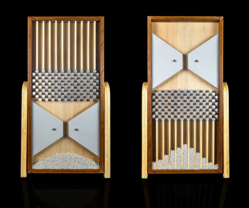
2.3 Pictures of centre and spread


2.4 Eight uses of averages and measures of spread
- Comparing groups fairly. The mean mark of two sections tells which section did better on average. The standard deviation tells which one is more mixed. A teacher at a Pokhara college can then plan extra classes for the more scattered section.
- Reporting the typical value of skewed data. Incomes, house prices and file sizes have a long right tail, so the mean overstates what is typical. The median is quoted instead, as in Nepal Living Standards Survey reports. Always state which average you used.
- Measuring the reliability of a system. A server with mean response time 80 ms but a huge spread feels slow to some users. Engineers report the median and the 95th percentile together. The percentile is a partition value from this unit.
- Quality control. A factory fills 500 g packets and tracks the mean and σ of the weights. A small σ means every packet is close to 500 g. If the mean drifts or σ grows, the machine is stopped and adjusted.
- Comparing unlike data with CV. The coefficient of variation is unitless, so it compares rupee prices and kilogram weights. A vegetable market whose tomato price has CV 30% is more unstable than rice at 5%. Traders and planners use this to judge risk.
- Grading and ranking. Percentiles show where a student stands among all candidates. Being at the 90th percentile in an entrance test means 90% scored lower. Admission offices, including TU's entrance units, rely on this idea.
- Detecting unusual values. Values far outside Q1 − 1.5 IQR or Q3 + 1.5 IQR are suspected outliers, as in the box plot of Figure 2.3. A bank flags a transaction ten times the customer's normal spread for checking. The same rule cleans sensor data.
- Feeding later methods. The mean and σ are the inputs of the normal distribution, confidence intervals and hypothesis tests in Units 4 to 7. A student who cannot compute them cannot do any later unit. They are the foundation of the whole subject.


Formula and fact sheet
- \bar{x} = \frac{\sum x}{n}; grouped \frac{\sum f x}{n}. Median = L + ( ( \frac{n}{2} − cf)/f)h. Mode = L + \left( \frac{d_{1}}{(d_{1} + d_{2})} \right) h.
- Q_{i} at position \frac{i (n + 1)}{4}. Range, Q D = \frac{(Q_{3} - Q_{1})}{2} ,\ M D = \frac{\sum |x - \bar{x}|}{n}.
- \sigma^{2} = \frac{\sum (x - \bar{x})^{2}}{n} = \frac{\sum x^{2}}{n} - \bar{x}^{2} ;\ s^{2} divides by n - 1. C V = \frac{\sigma}{\bar{x}} \times 100.
- Mean − mode ≈ 3 ( \mathrm{mean} − median). \sum (x - \bar{x}) = 0.
Chapter summary
- Mean, median and mode locate the centre; quartiles, deciles and percentiles split the data.
- Range, QD, MD, variance, standard deviation and CV measure spread; CV compares different data sets.
- The median resists outliers; the standard deviation is the standard measure of spread.
Practice
- Data: 4, 8, 6, 10, 12. Find the mean, median, population and sample standard deviation, and CV.
- For the frequency distribution in 2.1 find D_{6} (the 6th decile) and P_{90}.
- Why is the median preferred for income data?
- Two classes have means 70 and 55 with \sigma = 10 and 9. Which class is more consistent?
- State the effect on the mean and standard deviation if every mark is increased by 5 and then doubled.
- Prove \sum (x - \bar{x}) = 0.
- Compute the median of the data 3, 7, 7, 2, 9, 4.
Answers and worked solutions
1. Mean \frac{40}{5} = 8; ordered 4, 6, 8, 10, 12, median 8. Squared deviations 16 ,\ 0 ,\ 4 ,\ 4 ,\ 16 = 40: population variance 8 ,\ \sigma = 2.83; sample variance 10 ,\ s = 3.16; C V = 2.83 / 8 \times 100 = 35.4%.
2. D_{6}: \frac{6 n}{10} = 30 lies in 40–50 (cumulative 44; cf = 28): 40 + \frac{30 - 28}{16} \times 10 = 41.25. P_{90}: \frac{90 n}{100} = 45 lies in 50–60 (cf = 44 ,\ f = 6): 50 + \frac{45 - 44}{6} \times 10 = 51.67.
3. A few very high incomes pull the mean upward; the median is unaffected by extremes.
4. C V_{1} = \frac{10}{70} \times 100 = 14.3%; C V_{2} = \frac{9}{55} \times 100 = 16.4%. The first class is more consistent.
5. +5: mean + 5 ,\ \sigma unchanged; then \times 2: mean = 2 (\bar{x} + 5) ,\ \sigma = 2 \sigma.
6. \sum (x - \bar{x}) = \sum x - n \cdot \bar{x} = \sum x - \sum x = 0.
7. Ordered 2, 3, 4, 7, 7, 9: middle values 4 and 7 → 5.5.
Model answers: medium (5 marks) and long (10 marks) questions
Q1 (5 marks). The marks of 50 students are: 0-10: 4, 10-20: 10, 20-30: 18, 30-40: 12, 40-50: 6. Calculate the mean, median and mode.
Introduction. For grouped data the three averages use class midpoints and the class limits. We build a working table first.
| Class | f | Midpoint x | fx | Cumulative f |
|---|---|---|---|---|
| 0-10 | 4 | 5 | 20 | 4 |
| 10-20 | 10 | 15 | 150 | 14 |
| 20-30 | 18 | 25 | 450 | 32 |
| 30-40 | 12 | 35 | 420 | 44 |
| 40-50 | 6 | 45 | 270 | 50 |
Mean. \sum f x = 1310 and n = 50, so mean = 1310/50 = 26.2.
Median. \frac{n}{2} = 25 lies in the class 20-30 (cumulative 32), so L = 20, cf = 14 ,\ f = 18 ,\ h = 10. Median = 20 + \frac{25 - 14}{18} \times 10 = 26.11.
Mode. The modal class is 20-30 (f = 18). d_{1} = 18 - 10 = 8 and d_{2} = 18 - 12 = 6. Mode = 20 + \frac{8}{8 + 6} \times 10 = 25.71.
Check and conclusion. The empirical relation mean − mode ≈ 3 ( \mathrm{mean} − median) gives 0.49 against 0.27, so the data are only slightly skewed to the right (mean > median > mode, as in Figure 2.2). The typical student scored about 26 out of 50.
Q2 (5 marks). Two programs are timed. Program A has mean 50 ms and \sigma = 4 ms; program B has mean 20 ms and \sigma = 2.5 ms. Which one is more consistent? Explain the measure you use and why.
Introduction. Comparing σ directly would be unfair, because the two programs have different averages and σ is in the same unit as the data. We need a relative measure.
Coefficient of variation. C V = ( \sigma / mean) × 100%. It is unit-free, so it can compare data sets of different size or unit.
Calculation. For A: C V = \frac{4}{50} \times 100 = 8%. For B: C V = 2.5 / 20 \times 100 = 12.5%.
Interpretation. A smaller CV means less variation relative to the average. Program A varies by 8% of its mean, program B by 12.5%, so A is more consistent, even though its σ (4 ms) is larger than B's (2.5 ms).
Where it is used. Engineers compare the stability of two servers, investors compare the risk of two shares, and a planner compares rice prices (in rupees per kg) with fuel prices (in rupees per litre).
Conclusion Use σ when the data sets share one unit and mean; use CV when they do not.
Q3 (10 marks). Define dispersion. Explain range, quartile deviation, mean deviation, variance, standard deviation and coefficient of variation. Calculate all of them for the data 12, 15, 18, 20, 25, 30.
Introduction. Dispersion (spread, variation) shows how far the values scatter around their centre. Two classes can both average 20 marks, but in one every student is near 20 and in the other marks range from 0 to 40.
An average alone hides this, so a measure of dispersion always accompanies it (Figures 2.1 to 2.3).
The six measures.
- Range = maximum − minimum. It is quick but uses only two values and is spoiled by an outlier.
- Quartile deviation Q D = \frac{(Q_{3} - Q_{1})}{2}. It uses the middle 50% of data and ignores extremes.
- Mean deviation M D = \frac{\sum |x - \bar{x}|}{n}. It uses every value but absolute values are awkward in algebra.
- Variance \sigma^{2} = \frac{\sum (x - \bar{x})^{2}}{n}, in squared units. The sample form divides by n - 1.
- Standard deviation \sigma = \sqrt{\mathrm{variance}}, in the units of the data. It is the most important measure.
- Coefficient of variation C V = \frac{\sigma}{\bar{x}} × 100%, used to compare different data sets.
Calculation. n = 6 ,\ \sum x = 120, so \bar{x} = 20. Range = 30 - 12 = 18.
Using positions (n + 1)p, Q_{1} is the 1.75th item = 12 + 0.75 \times 3 = 14.25 and Q_{3} is the 5.25th item = 25 + 0.25 \times 5 = 26.25, so Q D = \frac{26.25 - 14.25}{2} = 6.
Absolute deviations are 8, 5, 2, 0, 5, 10 with sum 30, so M D = 5. Squared deviations are 64, 25, 4, 0, 25, 100 with sum 218, so variance = 218/6 = 36.33 and \sigma = 6.03. The sample variance is 218/5 = 43.6 and s = 6.60.
C V = 6.03 / 20 \times 100 = 30.14%. As a check, \frac{\sum x^{2}}{n} - \bar{x}^{2} = 2618/6 − 400 = 36.33.
Comparison (Table).
| Measure | Uses all values? | Affected by outliers? | Units | Best use |
|---|---|---|---|---|
| Range | no | very much | data | quick look |
| QD | no | no | data | skewed data |
| MD | yes | slightly | data | simple reports |
| Variance | yes | yes | squared | theory |
| σ | yes | yes | data | standard reporting |
| CV | yes | yes | none | comparing data sets |
Properties. Adding a constant to every value leaves every measure of spread unchanged; multiplying by c multiplies range, QD, MD and σ by |c|, and variance by c^{2}.
Conclusion. The data are moderately spread (\sigma \approx 6 around a mean of 20). Report the mean with σ for symmetric data, the median with QD for skewed data, and CV when two data sets must be compared.