Unit 2 · 9 teaching hours · 49 min read
Problem Solving Methods
What the syllabus asks for 8
- Formulating a search problem
- The example graph
- Uninformed (blind) search
- Informed (heuristic) search
- Local search and optimisation
- Constraint satisfaction problems
- Adversarial search and games
- Seeing the ideas: puzzles, people, games and traced searches
Find the quickest route from Kathmandu to Pokhara; solve a sliding-tile puzzle; colour a map with three colours so that no neighbours match; play tic-tac-toe perfectly.
These are very different problems with one structure in common: you have a start, a set of possible moves and a goal, and the answer is a sequence of moves.
This unit turns them into a graph and searches the graph, first blindly, then guided by a heuristic, then in the presence of an opponent. Every trace in this unit was produced by bca/tools/check_ai.py and the programs at the end.
- Problem formulation and the state space; measuring a search algorithm.
- Uninformed search: breadth-first, depth-first, uniform-cost, depth-limited, iterative deepening.
- Informed search: greedy best-first and A*, admissible and consistent heuristics; local search and simulated annealing.
- Constraint satisfaction problems and backtracking.
- Adversarial search: minimax and alpha–beta pruning.
2.1 Formulating a search problem
A well-defined problem has five components: the initial state; the actions available in each state; a transition model (the state produced by an action); a goal test; and a path cost (usually the sum of step costs).
A solution is a path from the initial state to a goal state; an optimal solution has the least cost. The set of all states reachable from the start is the state space, drawn as a graph whose nodes are states and edges are actions.
State: the position of the eight tiles and the blank (9!/2 = 181,440 reachable states). Initial state: any solvable arrangement. Actions: move the blank up, down, left or right.
Transition model: swap the blank with the neighbouring tile. Goal test: tiles in order. Path cost: 1 per move.
Half of the 9! = 362,880 arrangements are unreachable from any given start (parity), which is why a random arrangement may have no solution.
A search algorithm builds a search tree from the start by expanding nodes (generating their successors). The frontier (open list) holds nodes generated but not yet expanded; the explored set (closed list) prevents revisiting states.
Algorithms differ only in which frontier node is expanded next.
Measuring performance
| Criterion | Question |
|---|---|
| Completeness | If a solution exists, is it always found? |
| Optimality | Is the solution found the cheapest? |
| Time complexity | How many nodes are generated? |
| Space complexity | How many nodes are stored? |
Complexity uses b (branching factor, successors per node), d (depth of the shallowest goal) and m (maximum depth of the space).
2.2 The example graph
Most traces below use one small graph so that the algorithms can be compared directly. Edge costs: S–A 2, S–B 5, A–B 2, A–C 4, B–C 1, B–D 7, C–G 3, D–G 2. Start S, goal G. Where order matters, neighbours are taken alphabetically.
2.3 Uninformed (blind) search
These strategies use only the problem definition, with no knowledge of how promising a state is.
Breadth-first search (BFS)
Expand the shallowest node first, using a FIFO queue. Complete (if b is finite) and optimal when all step costs are equal. Time and space O(b^{d}): memory is the killer.
On the example graph BFS expands S, A, B, C, D, G and returns S → A → C → G with 3 edges but cost 9: it finds the path with the fewest steps, not the cheapest.
Depth-first search (DFS)
Expand the deepest node first, using a LIFO stack. Space is only O(b·m) and it finds deep solutions quickly, but it is not optimal and, in infinite or cyclic spaces without an explored set, not complete.
In the example the expansion order is S, A, B, C, G and the path S → A → B → C → G happens to cost 8; with a different neighbour order it would not.
Uniform-cost search (UCS)
Expand the node with the lowest path cost g(n) first (a priority queue); this is Dijkstra's algorithm. Complete and optimal for non-negative step costs.
In the example the nodes are expanded in the order S (0), A (2), B (4), C (5), G (8) and the optimal path S → A → B → C → G of cost 8 is found; note that B is reached first at cost 5 directly from S but later at cost 4 through A, and UCS keeps the cheaper.
Depth-limited and iterative deepening search
Depth-limited search is DFS with a depth limit l, which stops infinite descent but is incomplete if l < d. Iterative deepening DFS (IDDFS) repeats depth-limited search with l = 0, 1, 2, … until the goal is found, combining DFS's low memory with BFS's completeness and (for equal step costs) optimality.
The repeated work looks wasteful but is not, because most nodes are at the bottom level.
With b = 10 and d = 5, BFS generates 1 + 10 + 100 + 1,000 + 10,000 + 100,000 = 111,111 nodes, and IDDFS generates 6 + 5×10 + 4×100 + 3×1,000 + 2×10,000 + 1×100,000 = 123,456: only 11 % more.
On the example graph IDDFS succeeds at limit 3 with S → A → C → G.
| Algorithm | Complete | Optimal | Time | Space |
|---|---|---|---|---|
| BFS | yes | yes (equal costs) | O(b^{d}) | O(b^{d}) |
| DFS | no (cycles, infinite depth) | no | O(b^{m}) | O(b m) |
| UCS | yes | yes | O(b^{1 + C*/\varepsilon }) | same |
| Depth-limited | no if l < d | no | O(b^{l}) | O(b l) |
| IDDFS | yes | yes (equal costs) | O(b^{d}) | O(b d) |
Bidirectional search runs two searches (from start and from goal) that meet in the middle, giving O(b^{d/2}) each: for b = 10 and d = 6 that is about 2 × 1,000 nodes instead of 1,000,000.
2.4 Informed (heuristic) search
An evaluation function f(n) estimates the desirability of a node. A heuristic h(n) estimates the cheapest cost from n to a goal (h = 0 at the goal). The example graph's heuristic is h(S) = 6, h(A) = 5, h(B) = 3, h(C) = 2, h(D) = 2, h(G) = 0.
Greedy best-first search
f(n) = h(n): always expand the node that looks closest to the goal. Fast, but neither complete (it can loop) nor optimal. Here greedy expands S (6), B (3), C (2), G (0) and returns S → B → C → G with cost 9: it ignored the cost already paid.
A* search
f(n) = g(n) + h(n): the cost so far plus the estimated cost to go.
A* is complete and optimal if the heuristic is admissible (never overestimates: h(n) ≤ h*(n), the true remaining cost) for tree search, and consistent (monotone: h(n) ≤ c(n, n′) + h(n′) for every edge) for graph search.
Consistency implies admissibility and guarantees that f never decreases along a path, so the first time a node is expanded the path is optimal.
The true costs to the goal are h(S) = 8, h(A) = 6, h(B) = 4, h(C) = 3, h(D) = 2, so h ≤ h everywhere (admissible) and every edge satisfies h(n) ≤ c + h(n′) in both directions (consistent). The expansions:
| Expanded | g | h | f = g + h | Note |
|---|---|---|---|---|
| S | 0 | 6 | 6 | frontier: A (7), B (5 + 3 = 8) |
| A | 2 | 5 | 7 | B improves to g = 4, f = 7; C: g = 6, f = 8 |
| B | 4 | 3 | 7 | C improves to g = 5, f = 7; D: g = 11, f = 13 |
| C | 5 | 2 | 7 | G: g = 8, f = 8 |
| G | 8 | 0 | 8 | goal: path S → A → B → C → G, cost 8 |
A* found the optimum (8) where greedy found 9, expanding fewer nodes than UCS would on a large graph.
Designing heuristics: the 8-puzzle
Two classic admissible heuristics: h₁ = number of misplaced tiles and h₂ = sum of Manhattan distances of the tiles from their goal squares.
Both are exact costs of relaxed problems (tiles may jump anywhere; tiles may move onto occupied squares) and h₂ ≥ h₁, so h₂ dominates h₁ and is never worse.
For the start state 2 6 5 / 4 3 8 / 7 1 _ (goal 1 2 3 / 4 5 6 / 7 8 _), h₁ = 6 and h₂ = 12; the optimal solution has 16 moves.
A* expanded 144 nodes with h₂, 565 with h₁ and 8,166 with h = 0 (which is uniform-cost search): a better heuristic prunes more.
The hardest 8-puzzle positions need 31 moves; A* with Manhattan distance expands 21,198 nodes for one of them. The effective branching factor shows the same story: the better the heuristic, the nearer to 1.
If h₁ and h₂ are both admissible, so is max(h₁, h₂), and it dominates both. Heuristics can also come from pattern databases (exact costs of solving a subset of the tiles).
Memory-bounded variants
IDA* performs iterative deepening on the f-limit; RBFS and SMA* keep memory bounded. Weighted A* (f = g + w·h with w > 1) trades optimality for speed.
2.5 Local search and optimisation
When the path does not matter, only the final state does (n-queens, timetables, circuit layout), local search keeps a single current state and moves to neighbours, using constant memory.
- Hill climbing: move to the best neighbour; stop when none is better. It gets stuck on local maxima, plateaus and ridges. Remedies: random restarts, sideways moves, stochastic hill climbing.
- Simulated annealing: accept a worsening move of size ΔE with probability e^{-\Delta E/T}, and lower the temperature T slowly. At high T it explores (ΔE = 2 is accepted with probability e^{-2/10} = 0.8187 when T = 10); at low T it is nearly greedy (e^{-2/1} = 0.1353 when T = 1). With a slow enough cooling schedule it finds the global optimum with probability approaching 1.
- Local beam search keeps k states; genetic algorithms (Unit 4) combine pairs of states.
2.6 Constraint satisfaction problems
A CSP has variables X₁ … Xₙ, a domain for each and constraints over subsets. A solution assigns every variable a value satisfying all constraints. Because the structure is explicit, algorithms can reject whole branches early.
Variables: the regions WA, NT, SA, Q, NSW, V, T of the classic Australian map. Domain: {red, green, blue}. Constraints: neighbouring regions differ (WA–NT, WA–SA, NT–SA, NT–Q, SA–Q, SA–NSW, SA–V, Q–NSW, NSW–V).
With three colours there are exactly 18 solutions (6 for the mainland times 3 for isolated Tasmania); with two colours there are none, because WA, NT and SA form a triangle.
Backtracking search assigns one variable at a time and backtracks when a constraint is violated; in the fixed order WA, NT, SA, Q, NSW, V, T it makes a solution in 8 search nodes (the root plus 7 assignments) without ever having to backtrack. Better ordering and pruning:
- MRV (minimum remaining values): choose the variable with the fewest legal values (fail first).
- Degree heuristic: choose the variable involved in most constraints.
- Least-constraining value: try the value that rules out the fewest values for neighbours.
- Forward checking: after an assignment, delete inconsistent values from neighbours' domains; fail if a domain empties. Arc consistency (AC-3) goes further.
Other CSPs: Sudoku, scheduling exams so no student has two at once, assigning Nepali radio frequencies so near stations differ.
2.7 Adversarial search and games
In a two-player, zero-sum, perfect-information game (chess, tic-tac-toe) the players alternate. A game is defined by an initial state, the player to move, actions, a transition model, a terminal test and a utility (+1 win, 0 draw, −1 loss for MAX).
Minimax
MAX tries to maximise the utility, MIN to minimise it, and both play optimally. The minimax value of a node: the utility if terminal; the maximum of the children's values at a MAX node; the minimum at a MIN node.
The algorithm is a depth-first recursion; time O(b^{m}), space O(b m).
The tree is MAX (root) → two MIN nodes → each with two MAX nodes → each with two leaves: leaves 3, 5 | 6, 9 | 1, 2 | 0, −1. The lowest MAX nodes take maxima 5, 9, 2, 0; the MIN nodes take minima min(5, 9) = 5 and min(2, 0) = 0; the root takes max(5, 0) = 5.
Alpha–beta pruning
Keep two bounds: α (the best value MAX can already guarantee on the path) and β (the best MIN can guarantee). If at any node α ≥ β, the remaining children cannot influence the result and are pruned. The result is identical to minimax, with fewer nodes evaluated.
Evaluating left to right: the first MAX node reads 3, 5 and returns 5, so the first MIN node has β = 5. The second MAX node reads 6: α = 6 ≥ β = 5, so the leaf 9 is pruned. The root now has α = 5.
In the right subtree, the first MAX node reads 1 and 2 and returns 2, so the MIN node has β = 2; now α = 5 ≥ β = 2, so the whole MAX node (0, −1) is pruned. Value 5, with 5 of the 8 leaves examined (3, 5, 6, 1, 2).
A second example is the 2-ply tree MAX → three MIN nodes with leaves (3, 12, 8), (2, 4, 6), (14, 5, 2). Minimax gives min values 3, 2, 2 and root value 3.
With alpha–beta the leaves 3, 12, 8, 2, 14, 5, 2 are examined (7 of 9): after reading 2 in the second MIN node (2 < α = 3) the leaves 4 and 6 are skipped. A larger 27-leaf tree evaluates 22 leaves and returns the same value, 10.
With perfect move ordering alpha–beta examines O(b^{m/2}) nodes, effectively doubling the search depth (or letting b become √b).
Tic-tac-toe shows the effect: the complete game tree has 549,946 nodes (255,168 complete games) and minimax visits all of them, finding the value 0 (a draw with optimal play).
Alpha–beta with the plain left-to-right move order visits 18,297 nodes, about 3.3 % of that. Real game programs use an evaluation function at a depth cutoff, iterative deepening, transposition tables and good move ordering.
Stochastic games (backgammon) add chance nodes and use expectiminimax; Monte-Carlo tree search (AlphaGo) replaces the exact evaluation by random playouts.
Practising the commands
The first program runs the five search algorithms and A* on the example graph and prints the expansion order and path cost of each.
import heapq
from collections import deque
E = {("S","A"):2, ("S","B"):5, ("A","B"):2, ("A","C"):4, ("B","C"):1, ("B","D"):7, ("C","G"):3, ("D","G"):2}
G = {}
for (a, b), c in E.items(): G.setdefault(a, {})[b] = c; G.setdefault(b, {})[a] = c
H = {"S": 6, "A": 5, "B": 3, "C": 2, "D": 2, "G": 0}
cost = lambda p: sum(G[a][b] for a, b in zip(p, p[1:]))
def bfs():
    q = deque([["S"]]); seen = {"S"}; order = []
    while q:
        p = q.popleft(); order.append(p[-1])
        if p[-1] == "G": return p, order
        for m in sorted(G[p[-1]]):
            if m not in seen: seen.add(m); q.append(p + [m])
def dfs():
    st = [["S"]]; seen = set(); order = []
    while st:
        p = st.pop()
        if p[-1] in seen: continue
        seen.add(p[-1]); order.append(p[-1])
        if p[-1] == "G": return p, order
        for m in sorted(G[p[-1]], reverse=True):
            if m not in seen: st.append(p + [m])
def best_first(f):
    pq = [(f("S", 0), 0, ["S"])]; best = {}; order = []; tie = 0
    while pq:
        _, _, p = heapq.heappop(pq); n = p[-1]; g = cost(p)
        if n in best and best[n] <= g: continue
        best[n] = g; order.append((n, g))
        if n == "G": return p, order
        for m in sorted(G[n]):
            tie += 1; heapq.heappush(pq, (f(m, g + G[n][m]), tie, p + [m]))
for name, (path, order) in [("BFS", bfs()), ("DFS", dfs()), ("UCS", best_first(lambda n, g: g)),
                            ("Greedy", best_first(lambda n, g: H[n])), ("A*", best_first(lambda n, g: g + H[n]))]:
    print(f"{name:7s} path={'-'.join(path)} cost={cost(path)} expanded={order}")
BFS     path=S-A-C-G cost=9 expanded=['S', 'A', 'B', 'C', 'D', 'G']
DFS     path=S-A-B-C-G cost=8 expanded=['S', 'A', 'B', 'C', 'G']
UCS     path=S-A-B-C-G cost=8 expanded=[('S', 0), ('A', 2), ('B', 4), ('C', 5), ('G', 8)]
Greedy  path=S-B-C-G cost=9 expanded=[('S', 0), ('B', 5), ('C', 6), ('G', 9)]
A*      path=S-A-B-C-G cost=8 expanded=[('S', 0), ('A', 2), ('B', 4), ('C', 5), ('G', 8)]
The second program checks the minimax and alpha–beta examples and counts the nodes of the whole tic-tac-toe game tree with and without pruning.
import math
def minimax(t, maxp):
    if not isinstance(t, list): return t
    vals = [minimax(c, not maxp) for c in t]
    return max(vals) if maxp else min(vals)
seen = []
def alphabeta(t, maxp, a, b):
    if not isinstance(t, list): seen.append(t); return t
    v = -math.inf if maxp else math.inf
    for c in t:
        r = alphabeta(c, not maxp, a, b)
        if maxp: v = max(v, r); a = max(a, v)
        else: v = min(v, r); b = min(b, v)
        if a >= b: break
    return v
for tree in ([[[3, 5], [6, 9]], [[1, 2], [0, -1]]], [[3, 12, 8], [2, 4, 6], [14, 5, 2]]):
    seen.clear(); print("minimax", minimax(tree, True), "alpha-beta", alphabeta(tree, True, -math.inf, math.inf), "leaves read", seen)
LINES = [(0,1,2),(3,4,5),(6,7,8),(0,3,6),(1,4,7),(2,5,8),(0,4,8),(2,4,6)]
def winner(b):
    for x, y, z in LINES:
        if b[x] and b[x] == b[y] == b[z]: return b[x]
def solve(use_ab):
    count = [0]
    def rec(b, p, a, bt):
        count[0] += 1; w = winner(b)
        if w: return 1 if w == "X" else -1
        if all(b): return 0
        v = -2 if p == "X" else 2
        for i in range(9):
            if not b[i]:
                b[i] = p; r = rec(b, "O" if p == "X" else "X", a, bt); b[i] = None
                if p == "X": v = max(v, r); a = max(a, v)
                else: v = min(v, r); bt = min(bt, v)
                if use_ab and a >= bt: break
        return v
    return rec([None] * 9, "X", -2, 2), count[0]
print("tic-tac-toe minimax (value, nodes):", solve(False)); print("with alpha-beta:", solve(True))
minimax 5 alpha-beta 5 leaves read [3, 5, 6, 1, 2]
minimax 3 alpha-beta 3 leaves read [3, 12, 8, 2, 14, 5, 2]
tic-tac-toe minimax (value, nodes): (0, 549946)
with alpha-beta: (0, 18297)
2.8 Seeing the ideas: puzzles, people, games and traced searches
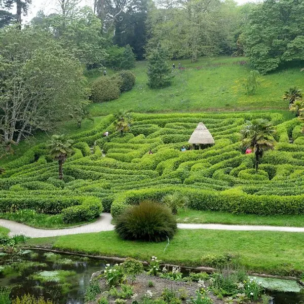
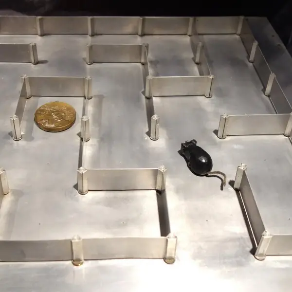
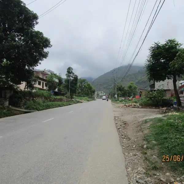
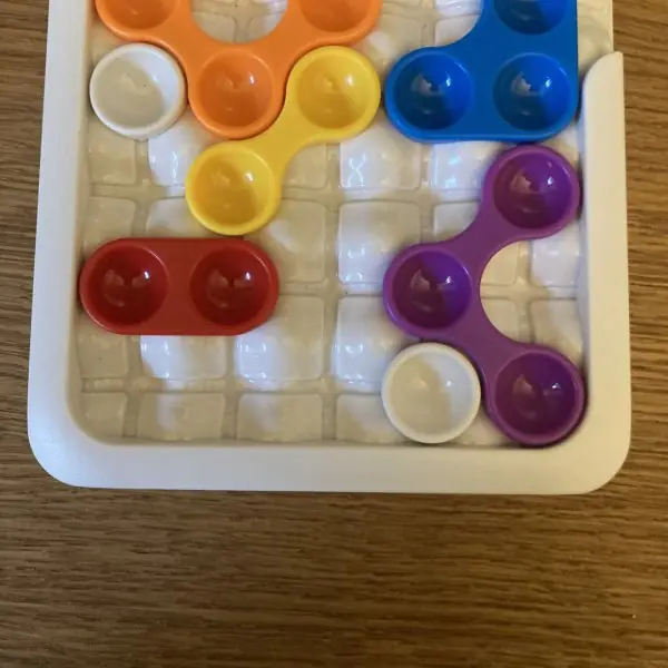
Search is easiest to understand when you can watch it run. Plate 2.1 shows four everyday search problems as real objects: a garden maze, Claude Shannon's maze-solving mouse, a country road between two towns and a sliding puzzle.
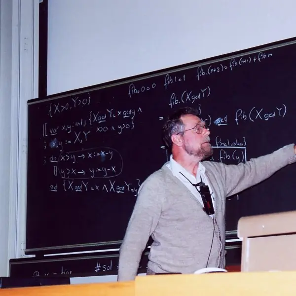
Plate 2.2 shows three people behind the algorithms of this unit: Edsger Dijkstra (shortest paths), Claude Shannon (the first chess-programming paper) and the Shakey team at SRI, where A* was invented.
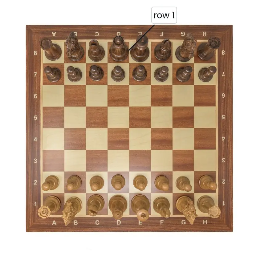
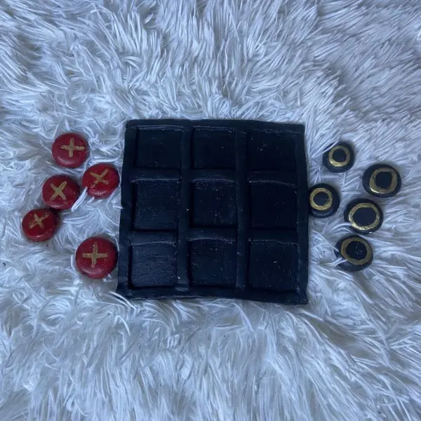
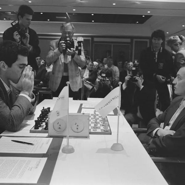
Plates 2.3 and 2.4 show the board games on which adversarial search is tested. Figures 2.1 to 2.11 then run the algorithms: every count, path and value printed on them is computed by the figure code itself.





2.8.1 Eight uses of search in Nepal
- Finding the way on a map. When you ask a map application for the best route from Kathmandu to Pokhara, it treats the roads as a weighted graph and searches it. The straight-line distance to the destination is an admissible heuristic, so A* can find the cheapest route while looking at only a small part of the national road network. Road closures, landslides and traffic change the edge costs, and the search is simply run again.
- Exam routines and class timetables. A university such as Tribhuvan University or a school must give every subject a room, a teacher and a time so that no student, teacher or room is used twice at once. This is a constraint satisfaction problem: the variables are the exams, the domains are the time slots and the constraints are the clashes. Backtracking with the most-constrained-first rule finds a valid routine quickly, and local search can then improve it, for example by spreading exams out.
- Delivery and ride dispatch. Food and parcel delivery companies and ride-hailing apps in Kathmandu must choose which rider takes which order and in what stop order. Finding the best order of many stops is the travelling-salesman problem, which is too large to solve exactly, so the apps use local search and heuristics to reach a very good route in a second. The result is a lower fuel cost and a shorter wait for the customer.
- Routing packets in networks. Internet providers and Nepal Telecom run link-state routing protocols in which every router runs Dijkstra's algorithm, the uniform-cost search of this unit, on a graph of links with costs. The result is a shortest-path tree that tells each router where to send each packet. When a link fails, the costs change and every router searches again, as the Networking book explains.
- Game-playing programs. Computer opponents in chess, Ludo or carrom-style games choose moves by minimax with alpha-beta pruning, looking a few moves ahead and scoring the positions with an evaluation function. Move ordering decides how many positions are pruned (Fig. 2.10), so good programs try the most promising moves first. A difficulty level in a game is often just the search depth.
- Puzzles and learning apps. Sudoku, sliding-tile and maze apps check a player's move or give a hint by searching the puzzle. Sudoku is a constraint problem like map colouring, and a sliding puzzle is solved with A* and the Manhattan-distance heuristic of Fig. 2.5. A hint is just the first step of the best solution found.
- Robot and drone navigation. A warehouse robot, a robot vacuum or a survey drone moves on a grid of free and blocked cells and plans a path around obstacles with A*, as in Fig. 2.4. Drone surveys of floods or landslides in hill districts use the same idea to plan flight lines that cover the area with the fewest turns. The path is recomputed when a new obstacle appears.
- Planning shifts, buses and resources. A hospital must give nurses and doctors shifts, and a bus company such as Sajha Yatayat must assign buses and drivers to routes, with rules about rest, skills and demand. These are large optimisation problems where the path does not matter, only the final plan, so local search and simulated annealing are used to improve the plan step by step. A planner accepts a slightly worse plan sometimes to escape a local maximum, exactly as in Fig. 2.6.
Formula and fact sheet
- BFS O(b^{d}) time and space; DFS O(b^{m}) time, O(bm) space; IDDFS O(b^{d}) time, O(bd) space. Nodes by BFS at b = 10, d = 5: 111,111; IDDFS: 123,456.
- UCS expands by g(n); greedy by h(n); A* by f(n) = g(n) + h(n).
- Admissible: h(n) ≤ h*(n). Consistent: h(n) ≤ c(n, n′) + h(n′). Consistent ⇒ admissible.
- Simulated annealing: accept a worse move with probability e^{-\Delta E/T}.
- Minimax value = max at MAX nodes, min at MIN nodes. Alpha–beta prunes when α ≥ β; best case O(b^{m/2}).
- CSP heuristics: MRV, degree, least-constraining value, forward checking, AC-3.
Chapter summary
- A search problem is defined by states, actions, a goal test and path costs; the algorithm determines which frontier node is expanded next.
- BFS, UCS and IDDFS are complete; BFS and IDDFS are optimal for equal step costs and UCS for any positive costs; DFS saves memory but is neither.
- A* with an admissible (tree) or consistent (graph) heuristic is optimal and more efficient than blind search; a dominant heuristic expands fewer nodes.
- Local search keeps one state and suits optimisation; simulated annealing escapes local maxima by occasionally accepting worse moves.
- CSPs are solved by backtracking with MRV and forward checking. Games are searched by minimax; alpha–beta gives the same answer with far fewer nodes.
Practice
- List the five components of a search problem and formulate the 8-puzzle.
- On the example graph, give the path and cost found by BFS, UCS, greedy and A*. Why does BFS not find the cheapest path?
- Why is IDDFS not wasteful? Compute the node counts for b = 10, d = 5.
- Define admissible and consistent heuristics. Show h is admissible on the example graph.
- For the 8-puzzle start 2 6 5 / 4 3 8 / 7 1 _ compute h₁ and h₂ and explain which dominates.
- Compare hill climbing and simulated annealing. What is the acceptance probability for ΔE = 2 at T = 1 and T = 10?
- Formulate Australia map colouring as a CSP. How many solutions with three colours?
- Apply minimax and alpha–beta to the tree with leaves 3, 5 | 6, 9 | 1, 2 | 0, −1 and state which leaves are pruned.
- Why does alpha–beta not change the minimax result? What is its best-case complexity?
- How many nodes are in the full tic-tac-toe tree, and what is the game's minimax value?
Answers and worked solutions
1. Initial state, actions, transition model, goal test, path cost. 8-puzzle: states are tile arrangements; actions move the blank; transition swaps blank and tile; goal is the ordered arrangement; cost 1 per move.
2. BFS: S → A → C → G, cost 9 (fewest edges). UCS: S → A → B → C → G, cost 8. Greedy: S → B → C → G, cost 9. A: S → A → B → C → G, cost 8. BFS counts steps, not costs.
3. Most nodes are at the deepest level, so the repeated shallow levels are cheap. BFS: 111,111 nodes; IDDFS: 6 + 50 + 400 + 3,000 + 20,000 + 100,000 = 123,456.
4. Admissible: h(n) never exceeds the true remaining cost; consistent: h(n) ≤ c(n, n′) + h(n′). On the example h = (S 8, A 6, B 4, C 3, D 2, G 0) and h = (6, 5, 3, 2, 2, 0) ≤ h, so it is admissible.
5. h₁ = 6 misplaced tiles; h₂ = 12 (Manhattan). h₂ ≥ h₁ for every state, so h₂ dominates and A expands fewer nodes (144 versus 565 in the test).
6. Hill climbing only improves and sticks in local maxima; annealing accepts worse moves with probability e^{-\Delta E/T}. For ΔE = 2: T = 1 gives 0.1353, T = 10 gives 0.8187.
7. Variables: seven regions; domain: three colours; constraints: adjacent regions differ. There are 18 solutions.
8. Minimax = 5. Alpha–beta prunes the leaf 9 (after 6, with α = 6 ≥ β = 5) and the subtree (0, −1) (after the right MIN node's β becomes 2 ≤ α = 5); 5 of 8 leaves are read.
9. A pruned branch cannot change the value at the root because MAX or MIN already has a better option elsewhere. Best case O(b^{m/2}).
10. 549,946 nodes (255,168 complete games); the value is 0 (draw). Alpha–beta with plain ordering visits 18,297 nodes.
Model answers for Unit 2
Q1. Explain the uninformed search strategies. Compare breadth-first, depth-first, uniform-cost and iterative-deepening search. (10 marks)
Introduction. Uninformed (blind) search strategies use only the problem definition: the states, the actions, the goal test and the step costs.
They have no idea which state is promising, and they differ only in which node of the frontier they expand next.
They are judged by completeness, optimality, time and space, using the branching factor b, the depth d of the shallowest goal and the maximum depth m.
The strategies.
- Breadth-first search (BFS) expands the shallowest node first with a FIFO queue (Fig. 2.2). It is complete and, when all step costs are equal, optimal, but it stores a whole level, so time and space are O(b^{d}). On the example graph it returns S-A-C-G of cost 9: the path with the fewest edges, not the cheapest (Fig. 2.1).
- Depth-first search (DFS) expands the deepest node first with a LIFO stack. Its memory is only O(b·m), but it is not optimal, and in a cyclic or infinite space without an explored set it may never finish.
- Uniform-cost search (UCS) expands the node with the smallest path cost g(n) using a priority queue; it is Dijkstra's algorithm. It is complete and optimal for positive step costs and returns S-A-B-C-G of cost 8.
- Depth-limited search is DFS with a depth limit l; it stops infinite descent but is incomplete when l < d.
- Iterative-deepening search (IDDFS) repeats depth-limited search with l = 0, 1, 2 and so on. It has the memory of DFS, O(b·d), and the completeness of BFS. The repeated work is small: for b = 10 and d = 8 it generates 123,456,789 nodes against 111,111,111 for BFS (Fig. 2.3).
Comparison.
| Algorithm | Complete | Optimal | Time | Space |
|---|---|---|---|---|
| BFS | yes | yes, if costs are equal | O(b^{d}) | O(b^{d}) |
| DFS | no | no | O(b^{m}) | O(b·m) |
| UCS | yes | yes | O(b^{1 + C*/\varepsilon }) | same |
| Depth-limited | no, if l < d | no | O(b^{l}) | O(b·l) |
| IDDFS | yes | yes, if costs are equal | O(b^{d}) | O(b·d) |
Memory is the real limit. At one million nodes per second and 1 KB per node, BFS to depth 10 needs 3.1 hours and 11.1 TB (Fig. 2.3), so it runs out of memory long before the user runs out of patience. Bidirectional search reduces the cost to about O(b^{d/2}).
Conclusion. Use BFS or IDDFS when costs are equal, UCS when costs differ, and DFS only when memory is tiny and any solution will do. All blind methods fail on large spaces, which is why heuristics are needed.
Q2. Explain A* search. What is an admissible heuristic? Trace A* on the example graph and compare it with greedy search. (10 marks)
Introduction. A* is the best-known informed search. It ranks frontier nodes by f(n) = g(n) + h(n), where g(n) is the cost already paid to reach n and h(n) is a heuristic estimate of the cheapest cost from n to a goal.
Using both parts balances the cost behind with the cost ahead.
Conditions for optimality. A heuristic is admissible if it never overestimates: h(n) ≤ h(n), the true remaining cost. A with an admissible heuristic is optimal for tree search.
A heuristic is consistent if h(n) ≤ c(n, n′) + h(n′) for every edge; this guarantees that f never decreases along a path, so the first time a node is expanded its path is optimal (graph search). Consistency implies admissibility.
Trace on the example graph (Fig. 2.1). With h(S) = 6, h(A) = 5, h(B) = 3, h(C) = 2, h(D) = 2 and h(G) = 0:
| Expanded | g | h | f | Frontier note |
|---|---|---|---|---|
| S | 0 | 6 | 6 | A (7), B (8) |
| A | 2 | 5 | 7 | B improves to g = 4, f = 7 |
| B | 4 | 3 | 7 | C improves to g = 5, f = 7 |
| C | 5 | 2 | 7 | G: g = 8, f = 8 |
| G | 8 | 0 | 8 | goal: S-A-B-C-G, cost 8 |
Comparison with greedy search. Greedy best-first search uses f(n) = h(n) alone.
On the same graph it expands S, B, C and G and returns S-B-C-G of cost 9: it is fast (4 expansions) but it ignores the cost already paid, so it is neither optimal nor complete in general.
A* needs 5 expansions and returns the optimal cost 8.
Effect of the heuristic. A better heuristic expands fewer nodes.
On the 8-puzzle start state of Fig. 2.5, uniform-cost search (h = 0) expands 7,495 nodes, A* with misplaced tiles (h1 = 6) expands 565 and A* with Manhattan distance (h2 = 12) expands 144, all finding the 16-move optimum.
On a grid with a wall, a heuristic that points into the wall helps much less (Fig. 2.4).
Conclusion. A* is complete and optimal with an admissible (tree) or consistent (graph) heuristic, and it is the standard choice for route finding; its weakness is memory, which IDA* and weighted A* reduce.
Q3. Explain minimax and alpha-beta pruning with an example. (10 marks)
Introduction. In a two-player game with perfect information, such as tic-tac-toe or chess, the best move depends on the reply of an opponent who is also trying to win.
Adversarial search models this with a game tree in which MAX (the player) and MIN (the opponent) move alternately.
Minimax. The value of a leaf is its utility for MAX (+1 win, 0 draw, -1 loss in tic-tac-toe). The value of a MAX node is the maximum of its children and the value of a MIN node is the minimum.
MAX picks the move whose child has the highest value, assuming MIN replies as well as possible. It is complete on a finite tree and optimal against an optimal opponent. Its time is O(b^{m}) and its space O(b·m).
Worked example (Fig. 2.9). For the tree with leaves 3, 5 | 6, 9 | 1, 2 | 0, -1, the lower MAX nodes are 5, 9, 2 and 0, the MIN nodes are 5 and 0, and the root is 5.
Alpha-beta pruning. Alpha is the best value MAX can already guarantee on the path and beta is the best value MIN can guarantee. A branch is cut as soon as α ≥ β, because the player above would never allow that position.
In Fig. 2.9 the leaf 9 is skipped (α = 6 ≥ β = 5) and the subtree 0, -1 is skipped (α = 5 ≥ β = 2). Five of eight leaves are read and the root is still 5.
| Method | Tic-tac-toe nodes | Note |
|---|---|---|
| Plain minimax | 549,946 | 255,168 complete games |
| Alpha-beta, order 0 to 8 | 18,297 | 96.7 percent saved |
| Alpha-beta, centre first | 7,275 | good ordering helps |
Complexity. With perfect ordering alpha-beta searches O(b^{m/2}) nodes, doubling the reachable depth. For games such as chess, programs also use a depth limit, an evaluation function and iterative deepening.
Conclusion. Alpha-beta returns exactly the minimax value with far fewer nodes, which is why it is the basis of game-playing programs.
Q4. What is a constraint satisfaction problem? Explain backtracking with map colouring. (10 marks)
Introduction. A constraint satisfaction problem (CSP) has variables X1 to Xn, a domain of values for each variable and constraints that restrict which combinations are allowed.
A solution assigns every variable a value so that all constraints hold. Because the structure is explicit, a solver can reject whole branches early instead of searching blindly.
Example (Fig. 2.8). Map colouring: the variables are the seven regions WA, NT, SA, Q, NSW, V and T, the domain is {red, green, blue} and the constraints say that neighbouring regions differ.
There are 3^{7} = 2,187 colourings and exactly 18 are valid. With two colours there is none, because WA, NT and SA form a triangle.
Backtracking search. It assigns one variable at a time, checks the constraints against the variables already assigned, and goes back to the previous variable when no value fits.
In the fixed order WA, NT, SA, Q, NSW, V, T with colours red, green, blue it finds a solution in 8 nodes without any backtracking: WA = red, NT = green, SA = blue, Q = red, NSW = green, V = red, T = red.
Improvements.
- Minimum remaining values (MRV) chooses the variable with the fewest legal values.
- Degree heuristic chooses the variable involved in the most constraints.
- Least-constraining value tries first the value that rules out the fewest choices for neighbours.
- Forward checking removes a value from a neighbour's domain when a variable takes it. After WA = red, NT = green and SA = blue, Q is forced to red (Fig. 2.8), and an empty domain would force an immediate backtrack.
- Arc consistency (AC-3) repeatedly removes values that have no support in a neighbouring variable.
| Method | Idea | Effect |
|---|---|---|
| Plain backtracking | assign, check, retreat | avoids bad branches |
| Forward checking | prune neighbour domains | detects dead ends early |
| MRV + degree | choose the hardest variable first | smaller tree |
Conclusion. CSP solvers combine backtracking with constraint propagation and variable-ordering heuristics, and they handle timetables, Sudoku and scheduling.
Q5. Compare hill climbing with simulated annealing. (5 marks)
Both are local search methods: they keep a single current state, use constant memory and are used when only the final state matters, such as timetables, n-queens or circuit layout.
Hill climbing moves to the best neighbour and stops when no neighbour is better. It is fast, but it stops at a local maximum, on a plateau or on a ridge.
On the landscape of Fig. 2.6, which has nine local maxima, hill climbing from 101 evenly spaced starting points reaches the highest peak only 19 times (18.8 percent).
Remedies are random restarts, sideways moves and stochastic hill climbing.
Simulated annealing also accepts a worse move of size ΔE with probability e^{-\Delta E/T}, where the temperature T is lowered slowly.
For ΔE = 2 the probability is 0.8187 at T = 10, so the search explores freely, and 0.1353 at T = 1, so it is almost greedy. In the same landscape, cooling from T = 3 reached the highest peak in 10 of 20 runs (50 percent).
With a slow enough cooling schedule it finds the global optimum with probability approaching 1.
| Hill climbing | Simulated annealing | |
|---|---|---|
| Moves accepted | only better | better always, worse with probability e^{-\Delta E/T} |
| Local maxima | gets stuck | can escape |
| Speed | very fast | slower, depends on cooling |
Q6. Explain heuristics for the 8-puzzle. Which one dominates? (5 marks)
A heuristic h(n) estimates the cost from a state to the goal. Good heuristics for the 8-puzzle come from relaxed problems, which are the puzzle with some rules removed.
If a tile may jump to any square, the exact cost is the number of misplaced tiles, h1.
If a tile may move onto an occupied neighbouring square, the exact cost is the sum of the Manhattan distances of the tiles from their goal squares, h2.
Because the relaxed cost can never exceed the real cost, both heuristics are admissible.
For the start state 2 6 5 / 4 3 8 / 7 1 _ and the goal 1 2 3 / 4 5 6 / 7 8 _, six tiles are misplaced, so h1 = 6, and the Manhattan distances 1, 2, 2, 0, 2, 2, 0 and 3 give h2 = 12 (Fig. 2.5). The optimal solution has 16 moves, and both values are below it.
h2 is never smaller than h1 for any state, so h2 dominates h1: A* with h2 expands no more nodes than A* with h1.
The experiment of Fig. 2.5 confirms it: uniform-cost search expands 7,495 nodes, A* with h1 expands 565 and A* with h2 expands 144.
If two admissible heuristics are available, max(h1, h2) is admissible and dominates both, and pattern databases can give even better estimates.
Q7. Define a well-defined search problem and formulate the 8-puzzle. How is the performance of a search algorithm measured? (5 marks)
A well-defined problem has five components. The initial state is where the agent starts. The actions are what the agent can do in each state. The transition model gives the state that results from an action.
The goal test checks whether a state is a goal. The path cost adds up the step costs along a path, and a solution is a path from the initial state to a goal state; it is optimal if its cost is the lowest.
For the 8-puzzle the state is the position of the eight tiles and the blank.
The initial state is any solvable arrangement, the actions move the blank up, down, left or right, the transition model swaps the blank with its neighbour, the goal test checks the order 1 to 8, and each move costs 1.
There are 9! = 362,880 arrangements, but only half, 181,440, are reachable from a given start, because of parity.
Performance is measured by four criteria: completeness (is a solution always found if one exists), optimality (is it the cheapest), time complexity (nodes generated) and space complexity (nodes stored).
They are expressed with the branching factor b, the depth d of the shallowest goal and the maximum depth m.
Q8. Distinguish between admissible and consistent heuristics with an example. (5 marks)
A heuristic h is admissible if it never overestimates the true cheapest remaining cost: h(n) ≤ h*(n) for every state n. It is consistent (or monotone) if for every state n and every successor n′ reached by an action of cost c(n, n′), h(n) ≤ c(n, n′) + h(n′).
This is a triangle inequality: the estimate from n is never more than the cost of one step plus the estimate from the next state.
Example. In the example graph of Fig. 2.1 the true costs to G are h(S) = 8, h(A) = 6, h(B) = 4, h(C) = 3, h(D) = 2 and h(G) = 0. The heuristic h = (6, 5, 3, 2, 2, 0) is below these values everywhere, so it is admissible.
It is also consistent: for the edge B-C of cost 1, h(B) = 3 ≤ 1 + h(C) = 3, and for A-B of cost 2, h(A) = 5 ≤ 2 + 3 = 5.
Why it matters. Every consistent heuristic is admissible, but not every admissible heuristic is consistent. For tree search, admissibility is enough for A* to be optimal.
For graph search with an explored set, consistency is needed: it guarantees that f(n) = g(n) + h(n) never decreases along a path, so the first time A* expands a node it has found the cheapest path to it and never has to reopen it.
Q9. Explain how the eight-queens problem is solved by backtracking. How many boards are examined? (5 marks)
The eight-queens problem asks for eight queens on a chessboard so that no two attack each other: no two share a row, a column or a diagonal.
It is a constraint satisfaction problem whose variables are the eight rows, whose values are the columns 1 to 8 and whose constraints forbid shared columns and diagonals.
A blind search that puts one queen in each row in any column examines 8^{8} = 16,777,216 boards. Insisting on different columns leaves 8! = 40,320 permutations.
Backtracking places one queen per row from row 1 downwards and tries the columns in order. Before placing a queen it checks the queens already on the board. If no column is safe, it goes back to the previous row and moves that queen.
The first solution found has queens in columns 1, 5, 8, 6, 3, 7, 2 and 4 (Plate 2.3).
Counted by the program of Fig. 2.7, backtracking visits only 2,057 nodes, including the empty board, to find all 92 solutions. Of these, only 12 are fundamentally different: the other 80 are rotations or reflections of those 12.
The saving comes from rejecting a whole group of boards as soon as the first two queens attack each other, which is the idea behind every constraint solver.