Unit 3 · 15 teaching hours · 53 min read
Knowledge Representation and Reasoning
What the syllabus asks for 6
- Knowledge and its importance
- Knowledge representation techniques
- Propositional logic
- First-order logic
- Reasoning under uncertainty
- Seeing the ideas: logicians, rules, networks and probabilities
Search can find a path through a graph someone has already drawn. But an intelligent system also needs to know things: that Socrates is a man, that all men are mortal, that an alarm may be triggered by a burglary or an earthquake.
This unit shows how knowledge is written down so that a program can reason with it: rules, semantic networks, frames, and above all logic, where reasoning becomes symbol manipulation that is guaranteed correct.
It ends with reasoning under uncertainty: Bayes' theorem and Bayesian networks.
- Knowledge: kinds, issues, properties of a good representation scheme.
- Techniques: rule-based systems, semantic nets, frames, logic.
- Propositional logic: syntax, semantics, entailment, inference rules, resolution.
- First-order logic: quantifiers, unification, resolution, forward and backward chaining.
- Uncertainty: probability, Bayes' rule, Bayesian networks.
3.1 Knowledge and its importance
Data is raw facts, information is data with meaning, and knowledge is information organised so that it can be used for decisions.
A program with a good algorithm and no knowledge of its domain is weak; many practical systems succeed because they hold a lot of knowledge about a narrow domain.
Types of knowledge
| Type | Meaning | Example |
|---|---|---|
| Declarative | facts about the world | Kathmandu is the capital of Nepal |
| Procedural | how to do something | the steps for long division |
| Meta-knowledge | knowledge about knowledge | which rule is most reliable |
| Heuristic | rules of thumb from experience | if the fever lasts more than three days, test for typhoid |
| Structural | relations between concepts | a bird is an animal; a wing is part of a bird |
Issues in knowledge representation
How do we represent attributes of objects and the relations between them (is-a, instance-of, part-of)? At what level of granularity do we represent knowledge?
How do we represent sets of objects and default knowledge that has exceptions (birds fly, but penguins do not)? How do we select the right structure when a problem arrives, and how do we keep knowledge consistent when it changes?
Properties of a good representation scheme
A good scheme has representational adequacy (it can express all the needed knowledge), inferential adequacy (new knowledge can be derived), inferential efficiency (the inference is fast) and acquisitional efficiency (knowledge can be added easily).
3.2 Knowledge representation techniques
Rule-based (production) systems
Knowledge is written as IF–THEN rules: IF engine does not start AND lights are dim THEN battery is flat.
A production system has a rule base, a working memory of current facts and an inference engine that matches rules to facts, selects one (conflict resolution) and fires it.
Rules are modular and easy to read, which is why they dominate expert systems (Unit 6); their weakness is slow matching in large rule sets and difficulty in representing structure.
Semantic networks
A semantic network is a graph: nodes are concepts and objects, labelled arcs are relations such as is-a and has-part. It supports inheritance: if Tweety is-a canary, canary is-a bird, and bird has wings, then Tweety has wings.
Questions are answered by following arcs. Limits: no standard meaning for arcs, awkward for negation and quantifiers, and exceptions need special handling.
Frames
A frame groups all the knowledge about an object or concept into slots (attributes) with facets: value, default, range, and attached procedures (if-needed, if-added, demons).
Frames are arranged in a class hierarchy with inheritance and defaults that sub-frames override.
Frame: Student            (is-a: Person)
  name:      [string]
  semester:  [1..8], default 1
  college:   default "unknown"
Frame: BCA-student        (is-a: Student)
  semester:  5            <- overrides the default
  credits:   if-needed: sum the credits of enrolled subjects
Frames are the ancestor of object-oriented programming.
Logic-based representation
Logic offers a formal language with a precise meaning and sound inference rules. It is the subject of the rest of this section.
3.3 Propositional logic
Syntax and semantics
A proposition is a statement that is either true or false. Atomic sentences are propositional symbols (P, Q, Rain). Complex sentences use the connectives ¬ (not), ∧ (and), ∨ (or), → (implies) and ↔ (if and only if).
A model assigns true or false to every symbol; the truth value of a sentence in a model comes from the truth tables.
| P | Q | ¬P | P ∧ Q | P ∨ Q | P → Q | P ↔ Q |
|---|---|---|---|---|---|---|
| F | F | T | F | F | T | T |
| F | T | T | F | T | T | F |
| T | F | F | F | T | F | F |
| T | T | F | T | T | T | T |
P → Q is false only when P is true and Q is false; it is equivalent to ¬P ∨ Q. A sentence is valid (a tautology) if true in all models, satisfiable if true in at least one, unsatisfiable if true in none.
Equivalences and entailment
De Morgan: ¬(P ∧ Q) ≡ ¬P ∨ ¬Q and ¬(P ∨ Q) ≡ ¬P ∧ ¬Q. Contrapositive: P → Q ≡ ¬Q → ¬P. Double negation: ¬¬P ≡ P. Distributivity of ∧ over ∨ and vice versa.
A knowledge base KB entails a sentence α (KB ⊨ α) if α is true in every model in which KB is true.
The simplest decision procedure is model checking by truth table: with n symbols there are 2ⁿ models (8 for the three symbols P, Q, R below).
Inference is sound if it derives only entailed sentences and complete if it derives all of them.
KB: P → Q, Q → R, P. Query: R. With three symbols there are 2³ = 8 models.
The only model that makes all three KB sentences true has P, Q and R all true, and R is true there, so KB ⊨ R. A frequent fallacy is affirming the consequent: from P → Q and Q one cannot conclude P (the model P false, Q true satisfies the KB), and the program below confirms KB ⊭ P.
Inference rules
- Modus Ponens: from α → β and α infer β.
- Modus Tollens: from α → β and ¬β infer ¬α.
- And-elimination: from α ∧ β infer α.
- Hypothetical syllogism: from α → β and β → γ infer α → γ.
- Resolution: from (α ∨ β) and (¬β ∨ γ) infer (α ∨ γ).
Conjunctive normal form and resolution
Resolution works on clauses (disjunctions of literals) and is refutation-complete: to prove KB ⊨ α, add ¬α to the KB, convert everything to CNF (a conjunction of clauses) and resolve pairs of clauses until the empty clause (a contradiction) appears; then the KB with ¬α is unsatisfiable, so KB ⊨ α.
Converting to CNF in four steps: (1) eliminate ↔ and → (α → β becomes ¬α ∨ β); (2) move ¬ inward with De Morgan; (3) remove double negations; (4) distribute ∨ over ∧.
Resolution refutation
Prove R from P → Q, Q → R and P. Clauses: (1) ¬P ∨ Q, (2) ¬Q ∨ R, (3) P. Negated query: (4) ¬R.
| Step | Resolve | Result |
|---|---|---|
| 5 | (3) P with (1) ¬P ∨ Q | Q |
| 6 | (5) Q with (2) ¬Q ∨ R | R |
| 7 | (6) R with (4) ¬R | empty clause ⊥ |
The empty clause shows the clauses are contradictory, so R follows from the KB.
The program below finds a refutation mechanically; because it saturates by trying every pair, its derivation takes more steps than the three-step proof above but ends at the same empty clause.
Horn clauses and chaining
A Horn clause has at most one positive literal: P₁ ∧ P₂ ∧ … ∧ Pₙ → Q (a rule), or a single fact. Most rule-based systems use Horn clauses because inference is linear in the size of the KB.
- Forward chaining (data-driven): start from known facts, fire every rule whose premises are satisfied, add the conclusion, repeat until the query is derived or nothing new appears. Good for monitoring and when many conclusions are wanted.
- Backward chaining (goal-driven): start from the query and look for rules that conclude it, then try to prove their premises as subgoals. Good for answering a specific question; it is how Prolog works.
For the rules A ∧ B → C, C → D, E → F and facts A, B: forward chaining derives C, then D; F is never derived (E is unknown). Backward chaining for D asks for C, then for A and B (known), and succeeds, without ever looking at the E rule.
3.4 First-order logic
Propositional logic cannot say "all men are mortal" without listing every man. First-order (predicate) logic (FOL) adds objects, predicates (relations) and functions, and the quantifiers ∀ (for all) and ∃ (there exists).
| Element | Examples |
|---|---|
| Constants | Socrates, Nepal, 5 |
| Variables | x, y |
| Predicates | Man(x), Loves(x, y), Greater(x, y) |
| Functions | Mother(x), Plus(x, y) |
| Connectives | ¬ ∧ ∨ → ↔ |
| Quantifiers | ∀x, ∃x |
Translating English to FOL
- "All men are mortal": ∀x (Man(x) → Mortal(x)). The natural connective with ∀ is → ; using ∧ would say everything is a man.
- "Some student passed": ∃x (Student(x) ∧ Passed(x)). The natural connective with ∃ is ∧ ; using → would be true if anything is not a student.
- "Every student likes some subject": ∀x (Student(x) → ∃y (Subject(y) ∧ Likes(x, y))).
- "No bird is a mammal": ∀x (Bird(x) → ¬Mammal(x)).
- Negation of quantifiers: ¬∀x P(x) ≡ ∃x ¬P(x) and ¬∃x P(x) ≡ ∀x ¬P(x). The order of mixed quantifiers matters: ∀x ∃y Loves(x, y) ("everyone loves someone") differs from ∃y ∀x Loves(x, y) ("someone is loved by everyone").
Inference in FOL
Universal instantiation replaces a ∀ variable by any constant: from ∀x Man(x) → Mortal(x) get Man(Socrates) → Mortal(Socrates).
Existential instantiation replaces ∃ by a fresh constant (a Skolem constant) or, when it depends on a universally quantified variable, a Skolem function. Generalised Modus Ponens uses unification.
Unification
Unification finds a substitution θ that makes two expressions identical.
Rules: a variable unifies with any term not containing it (the occurs check); a constant unifies only with itself; two predicates unify if they have the same name and their arguments unify, applying the substitution consistently.
| Pair | Unifier |
|---|---|
| Knows(John, x) and Knows(John, Jane) | {x / Jane} |
| Knows(John, x) and Knows(y, Mother(y)) | {y / John, x / Mother(John)} |
| P(A, B) and P(B, A) | fails (A and B are different constants) |
| Knows(John, x) and Knows(x, Jane) | fails unless the variables are standardised apart: rename one x to x′ and get |
The most general unifier (MGU) is the least restrictive substitution.
Resolution in FOL
- Convert to CNF: eliminate →, move ¬ inward, standardise variables apart, skolemise existentials, drop ∀, distribute ∨ over ∧.
- Negate the goal and add it.
- Resolve clauses with complementary literals that unify; apply the unifier to the resolvent.
- Stop when the empty clause appears.
Premises: (1) ∀x Man(x) → Mortal(x), (2) Man(Socrates). Goal: Mortal(Socrates).
CNF: (1) ¬Man(x) ∨ Mortal(x); (2) Man(Socrates); negated goal (3) ¬Mortal(Socrates).
Resolve (1) with (3) using {x / Socrates}: ¬Man(Socrates). Resolve that with (2): the empty clause. The goal is proved.
"Anyone who loves all animals is loved by someone. Jack loves all animals.
Is somebody loved by someone?" Skolemising ∃ introduces a function: for each x, a person f(x) who loves x. Unification binds variables to Jack and f(Jack), and resolution finds the contradiction with the negated goal.
The point of the exercise is the Skolem function: the lover depends on x.
Prolog
Prolog programs are Horn clauses and execution is backward chaining with unification and backtracking.
man(socrates).
man(plato).
mortal(X) :- man(X).
?- mortal(socrates).     % true
?- mortal(Who).          % Who = socrates ; Who = plato
Facts end with a period; :- means "if"; names starting with a capital are variables. Lists, recursion and unification make Prolog natural for rule-based and natural-language problems; the lab in this subject can use Prolog or LISP.
3.5 Reasoning under uncertainty
Logic assumes facts are true or false and known. Real agents face uncertainty from partial observability, noise and laziness (too many exceptions to list). Probability theory gives a degree of belief between 0 and 1.
Probability basics
- Axioms: 0 ≤ P(α) ≤ 1; P(true) = 1, P(false) = 0; P(α ∨ β) = P(α) + P(β) − P(α ∧ β).
- Conditional probability: P(α | β) = P(α ∧ β) / P(β).
- Product rule: P(α ∧ β) = P(α | β) P(β). Independence: P(α ∧ β) = P(α) P(β).
- Total probability: P(β) = Σ P(β | αᵢ) P(αᵢ).
- Bayes' rule: P(α | β) = P(β | α) P(α) / P(β).
A disease affects 1 % of a population. A test is positive for 95 % of sick people (sensitivity) and negative for 90 % of healthy ones (specificity), so 10 % of healthy people test positive.
P(positive) = 0.01 × 0.95 + 0.99 × 0.10 = 0.1085. By Bayes' rule P(disease | positive) = 0.01 × 0.95 / 0.1085 = 0.0876, only about 8.8 %, even though the test looks accurate.
The rarity of the disease (the prior) dominates: most positives are false positives.
Bayesian networks
A Bayesian network is a directed acyclic graph with a node for each random variable and, for each node, a conditional probability table (CPT) given its parents.
It represents the full joint distribution compactly: P(x₁, …, xₙ) = Π P(xᵢ | parents(xᵢ)). A joint over n Boolean variables needs 2ⁿ − 1 numbers; a network with at most k parents per node needs at most n·2ᵏ.
Burglary (B, prior 0.001) and Earthquake (E, prior 0.002) can set off the Alarm (A); two neighbours, John (J) and Mary (M), may call when they hear it.
CPT for A: P(A | B, E) = 0.95; P(A | B, ¬E) = 0.94; P(A | ¬B, E) = 0.29; P(A | ¬B, ¬E) = 0.001. John calls with P(J | A) = 0.90 and P(J | ¬A) = 0.05; Mary with P(M | A) = 0.70 and P(M | ¬A) = 0.01.
A full joint would need 2⁵ − 1 = 31 numbers; the network needs only 1 + 1 + 4 + 2 + 2 = 10.
One joint entry: P(j, m, a, ¬b, ¬e) = P(j | a) P(m | a) P(a | ¬b, ¬e) P(¬b) P(¬e) = 0.90 × 0.70 × 0.001 × 0.999 × 0.998 = 0.000628.
Inference by enumeration of P(B | j, m): sum the joint over the hidden variables E and A. P(b, j, m) = 0.000592; P(j, m) = 0.002084.
So P(B | j, m) = 0.000592 / 0.002084 = 0.2842: if both neighbours call, there is a 28 % chance of a burglary.
It is not higher because false alarms (earthquakes, or the neighbours' own mistakes) are common compared with the very rare burglary.
Inference algorithms: exact (enumeration, variable elimination) and approximate (sampling, Markov-chain Monte Carlo). Naive Bayes (Unit 4) is the simplest Bayesian network. Hidden Markov models and Kalman filters are Bayesian networks over time.
Decision under uncertainty
A utility function scores outcomes; a rational agent maximises expected utility: EU(a) = Σ P(outcome | a) U(outcome).
If the chance of rain is 0.3, an umbrella gives utility 70 when it rains and 80 when it does not, and no umbrella gives 0 when it rains and 100 when it does not: EU(umbrella) = 0.3 × 70 + 0.7 × 80 = 77, EU(no umbrella) = 0.7 × 100 = 70, so take the umbrella.
Other formalisms for uncertainty: certainty factors (MYCIN, Unit 6), fuzzy logic (degrees of truth such as "fairly hot" = 0.7) and Dempster–Shafer theory.
Practising the commands
The first program checks entailment by truth table, finds the resolution refutation mechanically and unifies the examples of this unit.
import itertools
imp = lambda a, b: (not a) or b
def entails(kb, q, syms):
    return all(q(m) for vals in itertools.product([False, True], repeat=len(syms))
               for m in [dict(zip(syms, vals))] if kb(m))
print("KB |= R:", entails(lambda m: imp(m["P"], m["Q"]) and imp(m["Q"], m["R"]) and m["P"], lambda m: m["R"], ["P", "Q", "R"]))
print("KB |= P (affirming the consequent):", entails(lambda m: imp(m["P"], m["Q"]) and m["Q"], lambda m: m["P"], ["P", "Q"]))
def resolve(c1, c2):
    out = []
    for l in c1:
        nl = l[1:] if l.startswith("~") else "~" + l
        if nl in c2: out.append(frozenset((c1 - {l}) | (c2 - {nl})))
    return out
clauses = [frozenset(c) for c in ({"~P", "Q"}, {"~Q", "R"}, {"P"}, {"~R"})]
derived = list(clauses); done = False
while not done:
    for a, b in itertools.combinations(list(derived), 2):
        for r in resolve(a, b):
            if r not in derived:
                derived.append(r); print("resolve", sorted(a), "+", sorted(b), "->", sorted(r) or "EMPTY CLAUSE")
                if not r: done = True; break
        if done: break
def is_var(x): return isinstance(x, str) and x in ("x", "y", "z")
def walk(x, s):
    while is_var(x) and x in s: x = s[x]
    return x
def unify(a, b, s):
    if s is False: return False
    a, b = walk(a, s), walk(b, s)
    if a == b: return s
    if is_var(a): return {**s, a: b}
    if is_var(b): return {**s, b: a}
    if isinstance(a, tuple) and isinstance(b, tuple) and len(a) == len(b):
        for x, y in zip(a, b):
            s = unify(x, y, s)
            if s is False: return False
        return s
    return False
print(unify(("Knows", "John", "x"), ("Knows", "John", "Jane"), {}))
print(unify(("Knows", "John", "x"), ("Knows", "y", ("Mother", "y")), {}))
print(unify(("P", "A", "B"), ("P", "B", "A"), {}))
KB |= R: True
KB |= P (affirming the consequent): False
resolve ['Q', '~P'] + ['R', '~Q'] -> ['R', '~P']
resolve ['Q', '~P'] + ['P'] -> ['Q']
resolve ['R', '~Q'] + ['~R'] -> ['~Q']
resolve ['Q', '~P'] + ['~Q'] -> ['~P']
resolve ['R', '~Q'] + ['Q'] -> ['R']
resolve ['Q'] + ['~Q'] -> EMPTY CLAUSE
{'x': 'Jane'}
{'y': 'John', 'x': ('Mother', 'y')}
False
The second program computes Bayes' rule for the medical test and enumerates the burglar-alarm network.
pd, sens, spec = 0.01, 0.95, 0.90
ppos = pd * sens + (1 - pd) * (1 - spec)
print("P(positive) = %.4f   P(disease | positive) = %.4f" % (ppos, pd * sens / ppos))
def joint(b, e, a, j, m):
    pb = .001 if b else .999; pe = .002 if e else .998
    pa = {(1, 1): .95, (1, 0): .94, (0, 1): .29, (0, 0): .001}[(b, e)]; pa = pa if a else 1 - pa
    pj = (.90 if a else .05) if j else (.10 if a else .95)
    pm = (.70 if a else .01) if m else (.30 if a else .99)
    return pb * pe * pa * pj * pm
print("P(j,m,a,~b,~e) = %.6f" % joint(0, 0, 1, 1, 1))
num = sum(joint(1, e, a, 1, 1) for e in (0, 1) for a in (0, 1))
den = sum(joint(b, e, a, 1, 1) for b in (0, 1) for e in (0, 1) for a in (0, 1))
print("P(b,j,m) = %.6f  P(j,m) = %.6f  P(B | j,m) = %.4f" % (num, den, num / den))
print("expected utility: umbrella", 0.3 * 70 + 0.7 * 80, " no umbrella", 0.7 * 100)
P(positive) = 0.1085   P(disease | positive) = 0.0876
P(j,m,a,~b,~e) = 0.000628
P(b,j,m) = 0.000592  P(j,m) = 0.002084  P(B | j,m) = 0.2842
expected utility: umbrella 77.0  no umbrella 70.0
3.6 Seeing the ideas: logicians, rules, networks and probabilities
Knowledge representation is abstract until you run it.
Plate 3.1 shows four figures behind logic: Aristotle (the syllogism), George Boole (algebra of true and false), Gottlob Frege (quantifiers and predicate logic) and Socrates, the man of the most famous syllogism.
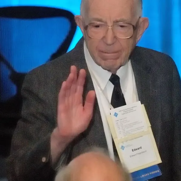
Plate 3.2 shows four people behind the tools of this unit: Alain Colmerauer (Prolog), Edward Feigenbaum (expert systems and rules), Marvin Minsky (frames) and Judea Pearl (Bayesian networks).
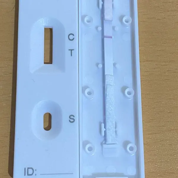
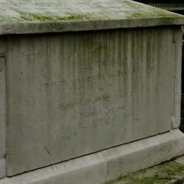
Plate 3.3 uses a canary and a penguin to show inheritance with exceptions, and Plate 3.4 shows the objects of the two uncertainty examples: a burglar alarm and a medical test, with the tomb of Thomas Bayes.
Figures 3.1 to 3.12 then run the ideas: every trace, truth value and probability is computed by the figure code.
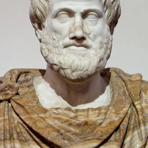
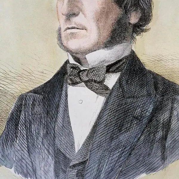
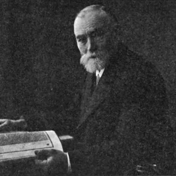
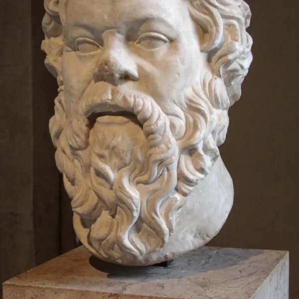









3.6.1 Eight uses of knowledge and reasoning in Nepal
- Farm advice by rules. A crop-advice service can store the knowledge of agriculture officers as IF-THEN rules, such as IF the leaves have yellow stripes AND the weather is cool and wet THEN suspect rust disease. A farmer answers a few questions by phone or app and the inference engine fires the matching rules, as in Fig. 3.1. The rules are easy for an expert to read and correct, which is why this style is used when the advice must be explained.
- Medical decision support. District hospitals and health posts use rapid tests for infections. As Fig. 3.10 shows, a positive result means different things in a village with many cases and in a town with few, so a good support tool combines the test with the local base rate using Bayes' rule. The tool suggests a confirmation test and leaves the decision to the health worker.
- Eligibility and rule checkers. Scholarship, tax and licence rules are written as conditions on age, income and documents. A program that holds them as rules can say yes or no and also explain which rule decided, which matters for fairness. This is forward chaining over a small fact base, and it avoids the errors of a clerk who forgets one clause.
- Spam and fraud filters. Banks and wallets such as eSewa, Khalti and Fonepay, and mail providers, estimate the probability that a message or payment is bad from signs such as the sender, amount and time. Each sign changes the belief by Bayes' rule, and naive Bayes (Unit 4) multiplies the evidence. The filter must keep false alarms low, because most payments are honest (the base-rate lesson of Fig. 3.10).
- Knowledge graphs and search. Facts such as Kathmandu is-a city, capital-of Nepal, part-of Bagmati Province are stored as a graph, a modern semantic network. A search engine uses the graph to answer a question directly and to find related pages, and inheritance lets it infer that a museum in Kathmandu is in Nepal. Wikipedia and Wikidata hold such facts for Nepali places and people.
- Chatbots with frames. A bank or telecom chatbot fills the slots of a frame, for example transfer: account, amount, receiver. It asks for each empty slot, uses defaults where it can and calls a procedure when the frame is full, as in Fig. 3.3. This keeps a conversation on track far better than free-form guessing.
- Flood and earthquake warning. Rainfall, river level, soil wetness and earlier floods are uncertain signs of a coming flood. A Bayesian network, like the alarm network of Fig. 3.11, combines them into one probability, and an agency such as the Department of Hydrology and Meteorology can decide when to warn villages along a river. The same method updates the chance of aftershocks.
- Decisions about risk. A bank decides on a loan, an insurer on a premium and a farmer on which crop to plant by comparing expected utility, as in Fig. 3.12. The best choice changes when the probability changes, so the numbers must be kept up to date. Such a model is a decision aid; it does not replace judgement about people.
Formula and fact sheet
- P → Q ≡ ¬P ∨ Q ≡ ¬Q → ¬P. De Morgan: ¬(P ∧ Q) ≡ ¬P ∨ ¬Q. n symbols give 2ⁿ models.
- Modus Ponens: α → β, α ⊢ β. Resolution: (α ∨ β), (¬β ∨ γ) ⊢ (α ∨ γ). Refutation: add ¬goal and derive the empty clause.
- FOL: ∀ goes with →, ∃ goes with ∧. ¬∀x P ≡ ∃x ¬P. Unify with the most general substitution.
- Forward chaining is data-driven; backward chaining is goal-driven (Prolog).
- Bayes: P(α | β) = P(β | α) P(α) / P(β). Network joint = Π P(xᵢ | parents).
- Expected utility EU(a) = Σ P(s | a) U(s).
Chapter summary
- Knowledge can be held as rules, semantic networks, frames or logic; a good scheme is adequate, inferentially efficient and easy to extend.
- Propositional logic gives sound, complete reasoning by truth table or resolution; Horn clauses allow efficient forward and backward chaining.
- First-order logic adds objects, relations and quantifiers; unification and resolution (with Skolemisation) prove theorems mechanically; Prolog implements the idea.
- Under uncertainty, probability and Bayes' rule update beliefs; Bayesian networks factor the joint distribution into small CPTs and answer queries by enumeration or sampling.
Practice
- Compare rules, semantic nets and frames for representing knowledge about vehicles.
- Build the truth table of P → Q and show it equals ¬P ∨ Q.
- Show by truth table that {P → Q, Q → R, P} entails R, and that {P → Q, Q} does not entail P.
- Prove R from {P → Q, Q → R, P} by resolution refutation.
- Translate:a"Every student who studies passes."b"Some student failed."c"No cat is a dog."
- Unify Knows(John, x) with Knows(y, Mother(y)); explain why P(A, B) and P(B, A) do not unify.
- Prove Mortal(Socrates) from ∀x Man(x) → Mortal(x) and Man(Socrates) by resolution.
- With rules A ∧ B → C, C → D, E → F and facts A, B, show forward and backward chaining for D.
- A test with 95 % sensitivity and 90 % specificity is applied to a 1 % prevalence disease. Find P(disease | positive).
- For the burglar-alarm network compute P(j, m, a, ¬b, ¬e) and explain why P(B | j, m) is only 0.28.
- How many numbers does the alarm network need compared with the full joint?
Answers and worked solutions
1. Rules: IF has-wheels AND has-engine THEN motor-vehicle (modular, no structure). Semantic net: Car is-a Vehicle, Vehicle has-part Wheel (inheritance, no precise semantics). Frame: Car with slots wheels = 4, fuel, owner, default values, inherited from Vehicle.
2. Rows (P, Q): FF → T, FT → T, TF → F, TT → T. ¬P ∨ Q has the same four values.
3. Only the row P = Q = R = true satisfies the KB and R is true there, so R is entailed. For {P → Q, Q}: the model P = false, Q = true satisfies the KB but not P, so P is not entailed.
4. Clauses ¬P ∨ Q, ¬Q ∨ R, P, ¬R. Resolve P with ¬P ∨ Q to get Q; Q with ¬Q ∨ R to get R; R with ¬R to get the empty clause.
5.(a) ∀x (Student(x) ∧ Studies(x) → Passes(x)).(b) ∃x (Student(x) ∧ Failed(x)).(c) ∀x (Cat(x) → ¬Dog(x)).
6. {y / John, x / Mother(John)}. P(A, B) and P(B, A) require A = B, but they are distinct constants, so unification fails.
7. Clauses ¬Man(x) ∨ Mortal(x), Man(Socrates), ¬Mortal(Socrates). Resolving the first and third with {x / Socrates} gives ¬Man(Socrates); with Man(Socrates) it gives the empty clause.
8. Forward: from A, B fire A ∧ B → C, then C → D; the E rule never fires. Backward: D needs C (rule C → D); C needs A and B (rule A ∧ B → C); both are facts, so D is proved.
9. P(positive) = 0.01 × 0.95 + 0.99 × 0.10 = 0.1085; P(disease | positive) = 0.0095 / 0.1085 = 0.0876.
10. 0.90 × 0.70 × 0.001 × 0.999 × 0.998 = 0.000628. P(B | j, m) = 0.000592 / 0.002084 = 0.2842: burglaries are very rare (0.001), so even two calls leave false alarms as the more probable explanation in most cases.
11. The network: 1 + 1 + 4 + 2 + 2 = 10 numbers; the full joint over five Boolean variables: 2⁵ − 1 = 31.
Model answers for Unit 3
Q1. Explain the main techniques of knowledge representation. What makes a good representation scheme? (10 marks)
Introduction. Knowledge is information organised so that a program can use it for decisions. A knowledge representation scheme is a language for writing that knowledge down together with procedures that derive new knowledge from it.
The kinds to be represented include declarative facts, procedural know-how, heuristic rules of thumb and structural relations between concepts.
Main techniques.
- Rule-based (production) systems store knowledge as IF-THEN rules in a rule base, with the known facts in a working memory. An inference engine matches rules to facts, chooses one by conflict resolution and fires it (Fig. 3.1). Rules are modular and easy to read, which is why expert systems use them, but matching is slow in very large rule bases.
- Semantic networks are graphs in which nodes are concepts and labelled arcs such as is-a and has-part are relations. They support inheritance: Tweety is-a canary, canary is-a bird, so Tweety has the wings and the default flight of a bird (Fig. 3.2). Their weakness is that arcs have no standard meaning and negation and quantifiers are awkward.
- Frames group the slots of an object, each with a value, a default, a range or an attached procedure, in a class hierarchy (Fig. 3.3). Sub-frames override defaults, and an if-needed procedure computes a slot when it is asked for. Frames are the ancestor of classes in object-oriented programming.
- Logic gives a formal language with exact meaning and sound inference. Propositional logic handles true and false statements, and first-order logic adds objects, predicates and quantifiers.
| Technique | Strength | Weakness |
|---|---|---|
| Rules | modular, explainable | slow for huge rule sets |
| Semantic nets | visual, inheritance | no precise semantics |
| Frames | defaults, procedures | rigid structure |
| Logic | precise, sound inference | hard to state uncertain knowledge |
Properties of a good scheme. It needs representational adequacy (it can express all the needed knowledge), inferential adequacy (it can derive new knowledge), inferential efficiency (inference is fast) and acquisitional efficiency (knowledge is easy to add).
Conclusion. No single scheme is best; practical systems combine rules, hierarchies and logic, and add probability when knowledge is uncertain.
Q2. Explain propositional logic: syntax, semantics, equivalences and entailment, with an example. (10 marks)
Introduction. Propositional logic is the simplest logic. A proposition is a statement that is either true or false, and sentences are built from propositional symbols with five connectives. It is the base on which first-order logic and resolution are built.
Syntax. Atomic sentences are symbols such as P, Q and Rain. Complex sentences use ¬ (not), ∧ (and), ∨ (or), → (implies) and ↔ (if and only if), with brackets.
Semantics. A model assigns true or false to every symbol, and the value of a sentence in that model follows the truth tables (Fig. 3.4).
The implication P → Q is false only when P is true and Q is false, and it is equivalent to ¬P ∨ Q. A sentence is valid if it is true in every model, satisfiable if it is true in at least one and unsatisfiable if it is true in none.
Equivalences. Machine checking over every model confirms that P → Q ≡ ¬P ∨ Q, that P → Q ≡ ¬Q → ¬P (contrapositive), and the two De Morgan laws ¬(P ∧ Q) ≡ ¬P ∨ ¬Q and ¬(P ∨ Q) ≡ ¬P ∧ ¬Q. The converse Q → P is not equivalent to P → Q.
Entailment. A knowledge base KB entails a sentence α, written KB ⊨ α, if α is true in every model in which KB is true. For n symbols there are 2ⁿ models, which is 8 for three symbols but more than a billion for thirty.
Example (Fig. 3.5). Let KB = {P → Q, Q → R, P} and the query R. Among the 8 models only the one with P, Q and R all true makes the whole KB true, and R is true in it, so KB ⊨ R. For KB = {P → Q, Q} the models P false, Q true and P true, Q true both satisfy it, so P is not entailed: this is the fallacy of affirming the consequent.
Inference rules. Modus ponens infers β from α → β and α; modus tollens infers ¬α from α → β and ¬β; hypothetical syllogism chains α → β and β → γ; and-elimination infers α from α ∧ β. They are sound: they derive only entailed sentences.
Conclusion. Propositional logic is exact and decidable, but truth tables grow exponentially, so resolution and chaining are used for large knowledge bases.
Q3. Explain resolution in propositional logic. Convert sentences to CNF and prove R from P → Q, Q → R and P. (10 marks)
Introduction. Resolution is a single inference rule that is sound and refutation-complete: if a set of clauses is unsatisfiable, resolution will derive the empty clause. It works on clauses, which are disjunctions of literals, and it proves a query by contradiction.
The rule. From (α ∨ β) and (¬β ∨ γ) infer (α ∨ γ). Two clauses that contain complementary literals are resolved by cancelling the pair and joining what remains. Resolving P with ¬P gives the empty clause, a contradiction.
Conversion to conjunctive normal form (CNF).
- Eliminate ↔ and → : replace α → β by ¬α ∨ β.
- Move ¬ inward with De Morgan's laws.
- Remove double negations.
- Distribute ∨ over ∧ so that the result is a conjunction of clauses.
Refutation procedure. To prove KB ⊨ α, add ¬α to the clauses of KB, resolve pairs of clauses and add the resolvents, and stop when the empty clause appears. If it appears, KB together with ¬α is unsatisfiable, so KB entails α.
Worked proof (Fig. 3.6). The clauses are (1) ¬P ∨ Q, (2) ¬Q ∨ R, (3) P, and the negated query (4) ¬R.
| Step | Resolve | Result |
|---|---|---|
| 5 | (3) P with (1) ¬P ∨ Q | Q |
| 6 | (5) Q with (2) ¬Q ∨ R | R |
| 7 | (6) R with (4) ¬R | empty clause |
The empty clause is a contradiction, so R follows from the knowledge base. A program that resolves every pair until nothing new appears also reaches the empty clause, but it derives many useless clauses on the way.
Why it works. Suppose the knowledge base is true and the query R is false.
Then clauses (1) to (4) would all be true in one model, but resolution is sound, so every clause it derives is true in that model, and the empty clause is never true.
Because the empty clause is derived, no such model exists: whenever the knowledge base is true, R must be true.
This is proof by contradiction, and it is why resolution needs only one rule instead of the many inference rules of natural deduction.
In practice programs add control strategies, such as always resolving with the shortest clause, to avoid deriving clauses that cannot help.
Conclusion. Resolution reduces reasoning to one mechanical rule on clauses, and Horn clauses allow a faster special case, chaining.
Q4. Explain first-order logic: syntax, quantifiers, English translation, unification and resolution. (10 marks)
Introduction. Propositional logic cannot say that all men are mortal without listing every man. First-order logic (FOL) adds objects, predicates and functions, and the quantifiers ∀ (for all) and ∃ (there exists), so one sentence can speak about many objects.
Syntax. The elements are constants (Socrates), variables (x, y), predicates (Man(x), Loves(x, y)), functions (Mother(x)), the five connectives and the two quantifiers.
Translation rules. The natural connective with ∀ is → and with ∃ is ∧ (Fig. 3.8). "All students passed" is ∀x (Student(x) → Passed(x)); writing ∧ would say that everyone is a student who passed, which is false whenever there is a teacher. "Some student passed" is ∃x (Student(x) ∧ Passed(x)); writing → would be true whenever anything is not a student, even if no student passed. Also ¬∀x P(x) ≡ ∃x ¬P(x).
Unification. To resolve in FOL we need a substitution that makes two literals identical. Knows(John, x) and Knows(y, Mother(y)) unify with {y/John, x/Mother(John)}, the most general unifier (Fig. 3.9).
P(A, B) and P(B, A) fail because the constants differ, and a variable cannot be bound to a term that contains itself (occurs check).
Resolution in FOL. Convert to CNF, standardise the variables apart, replace each ∃ by a Skolem constant or function, drop the ∀, add the negated goal, and resolve literals that unify until the empty clause appears.
Example. Premises: ¬Man(x) ∨ Mortal(x) and Man(Socrates); negated goal ¬Mortal(Socrates). Resolving the first and the goal with {x/Socrates} gives ¬Man(Socrates), and resolving that with Man(Socrates) gives the empty clause, so Mortal(Socrates) is proved.
Comparison.
| Propositional logic | First-order logic | |
|---|---|---|
| Objects | none, only true or false symbols | constants, variables, functions |
| Relations | no | predicates such as Man(x) |
| General statements | must list every case | ∀ and ∃ in one sentence |
| Inference | truth tables, resolution | unification with resolution |
The price of this power is that FOL entailment is only semi-decidable: a proof is found if the sentence is entailed, but the search may never finish if it is not.
Conclusion. FOL is far more expressive than propositional logic, and unification with resolution lets a program prove theorems; Prolog applies the idea to Horn clauses.
Q5. What is a Bayesian network? Explain with the burglar-alarm example. (10 marks)
Introduction. Real knowledge is uncertain. A Bayesian network is a directed acyclic graph in which each node is a random variable and each node has a conditional probability table (CPT) given its parents.
It represents the full joint distribution compactly: P(x₁, …, xₙ) = Π P(xᵢ | parents(xᵢ)).
The example (Fig. 3.11). Burglary B (prior 0.001) and Earthquake E (prior 0.002) can set off the Alarm A; John (J) and Mary (M) may call when they hear it.
The CPT of A is P(a | b, e) = 0.95, P(a | b, ¬e) = 0.94, P(a | ¬b, e) = 0.29 and P(a | ¬b, ¬e) = 0.001; John calls with probability 0.90 if the alarm sounds and 0.05 if not, and Mary with 0.70 and 0.01.
Compact representation. The full joint over five Boolean variables needs 2⁵ − 1 = 31 numbers, but the network needs 1 + 1 + 4 + 2 + 2 = 10. The saving grows quickly with more variables if each node has few parents.
Computing a joint entry. P(j, m, a, ¬b, ¬e) = P(j | a) P(m | a) P(a | ¬b, ¬e) P(¬b) P(¬e) = 0.90 × 0.70 × 0.001 × 0.999 × 0.998 = 0.000628.
Inference by enumeration. To find P(B | j, m) sum the joint over the hidden variables E and A: P(b, j, m) = 0.000592 and P(j, m) = 0.002084, so P(B | j, m) = 0.000592 / 0.002084 = 0.2842.
Even when both neighbours call, the chance of a burglary is only 28 percent, because burglaries are rare and false alarms from earthquakes or mistaken neighbours are common.
Reading the network. The arrows show the causes: the alarm depends on burglary and earthquake only, and John and Mary depend on the alarm only, so given the alarm they are independent of the burglary itself.
This is the independence assumption that makes the small tables enough.
The result also shows explaining away: if the neighbours call and we then learn that an earthquake happened, the probability of a burglary falls, because the earthquake already explains the alarm.
| Method | Idea |
|---|---|
| Enumeration | sum the joint over hidden variables |
| Variable elimination | reuse partial sums |
| Sampling (MCMC) | approximate by random samples |
Conclusion. Bayesian networks factor a large joint distribution into small tables and answer queries by exact or approximate inference.
Q6. Distinguish forward chaining from backward chaining with an example. (5 marks)
Both methods use Horn clauses, rules with one conclusion and several premises.
Forward chaining is data-driven: it starts from the known facts, fires every rule whose premises are all known, adds the conclusion to the facts and repeats until the query is derived or nothing new appears.
It suits monitoring systems and cases where many conclusions are wanted. Backward chaining is goal-driven: it starts from the query, finds a rule that concludes it and tries to prove the premises as subgoals.
It suits answering one question and is how Prolog works.
Example (Fig. 3.7). Rules: A ∧ B → C, C → D, E → F. Facts: A and B. Forward chaining fires A ∧ B → C, then C → D, and derives C and D; E → F never fires because E is unknown, so F is not derived.
Backward chaining for D uses the rule C → D and asks for C; the rule A ∧ B → C asks for A and B, which are facts, so D is proved after looking at only two rules and without touching the E rule.
| Forward | Backward | |
|---|---|---|
| Starts from | facts | the query |
| Direction | data-driven | goal-driven |
| May waste work on | irrelevant facts | repeated subgoals |
Q7. Explain Bayes' rule with the example of a medical test. (5 marks)
Bayes' rule updates a belief from evidence: P(α | β) = P(β | α) P(α) / P(β), where P(α) is the prior probability and P(β) comes from the total probability P(β) = Σ P(β | αᵢ) P(αᵢ).
Example (Fig. 3.10). A disease affects 1 percent of a population. The test is positive for 95 percent of the sick (sensitivity) and for 10 percent of the healthy (false-positive rate).
In 10,000 people, 100 are sick and 95 of them test positive; 9,900 are healthy and 990 of them test positive. The probability of a positive result is P(positive) = 0.01 × 0.95 + 0.99 × 0.10 = 0.1085, which is 1,085 people in 10,000.
By Bayes' rule P(disease | positive) = 0.01 × 0.95 / 0.1085 = 0.0876.
So a positive result means only an 8.8 percent chance of disease, although the test looks accurate. The reason is the base rate: healthy people outnumber the sick 99 to 1, so false alarms outnumber true positives.
If the same test were used where 10 percent are sick, the probability would rise to 51.4 percent. A test result must always be read together with how common the disease is.
Q8. Compare semantic networks with frames. (5 marks)
A semantic network is a graph in which nodes are concepts or objects and labelled arcs are relations such as is-a, instance-of and has-part.
Knowledge is found by following arcs, and inheritance passes properties down the is-a links: Tweety is-a canary and canary is-a bird, so Tweety inherits has = wings (Fig. 3.2).
An exception is handled by putting the value lower in the hierarchy: the nearest value wins, so Penguin overrides the can-fly = yes of Bird with can-fly = no.
A frame collects all the knowledge about one concept in named slots.
A slot can hold a value, a default, a range or an attached procedure: an if-needed procedure computes the value when it is asked for, an if-added procedure runs when a value is stored, and a demon reacts to a change.
Frames are arranged in a class hierarchy, and an instance frame inherits the slots of its class (Fig. 3.3), such as the credits that are computed for a student.
| Semantic network | Frame | |
|---|---|---|
| Unit of knowledge | node and arcs | slots in one structure |
| Procedures | no | yes (if-needed, demons) |
| Defaults | by position in the graph | explicit default facet |
| Descendant | knowledge graphs | object-oriented classes |
Both support inheritance and defaults, but frames add structure and procedures.
Q9. What is unification? Unify Knows(John, x) with Knows(y, Mother(y)). (5 marks)
Unification finds a substitution of terms for variables that makes two logical expressions identical. It is the step that lets resolution and Prolog match a general rule with a specific fact.
The substitution θ is the most general unifier (MGU) if every other unifier is a special case of it, so it commits to as little as possible.
Algorithm. Compare the two expressions argument by argument. If they are equal, nothing is needed. If one is a variable, bind it to the other term, provided the variable does not occur inside that term (occurs check).
If both are compound terms, the function symbols and the number of arguments must match, and the arguments are unified in turn with the bindings so far. Otherwise unification fails.
Worked example (Fig. 3.9). In Knows(John, x) and Knows(y, Mother(y)) the first arguments John and y give y = John. The second arguments x and Mother(y) give x = Mother(y), which becomes x = Mother(John) after applying y = John. The MGU is {y/John, x/Mother(John)}.
Failures. P(A, B) and P(B, A) fail because the constants A and B differ. Knows(John, x) and Knows(x, Jane) fail because x cannot be both John and Jane; after standardising apart (renaming one x to x₁) they unify with {x₁/John, x/Jane}.
P(x) and P(f(x)) fail the occurs check.
Q10. What is expected utility? How does a rational agent choose under uncertainty? (5 marks)
A utility function gives each outcome a number that says how desirable it is, and the expected utility of an action is the sum over its possible outcomes of the probability of the outcome times its utility: EU(a) = Σ P(outcome | a) U(outcome).
A rational agent chooses the action with the highest expected utility. This combines probability theory, which says what is likely, with utility theory, which says what is wanted.
Example (Fig. 3.12). The chance of rain is 0.3. An umbrella gives utility 70 if it rains and 80 if it does not; no umbrella gives 0 if it rains and 100 if it does not.
Then EU(umbrella) = 0.3 × 70 + 0.7 × 80 = 77 and EU(no umbrella) = 0.7 × 100 = 70, so the agent takes the umbrella.
Sensitivity. With rain probability p, EU(umbrella) = 80 − 10p and EU(no umbrella) = 100 − 100p. The two are equal at p = 2/9 = 0.2222, so the umbrella is better whenever rain is more than 22 percent likely.
The decision therefore depends on the probability as well as on the utilities, which is why a loan decision or a flood warning must be re-evaluated when the probabilities change.