Graphs and Trees

Graphs model networks of every kind: roads, the Internet, social ties, compiler flow, dependencies between tasks. Trees are the graphs that organise data (file systems, parse trees, search trees).

This unit gives the vocabulary, the key theorems and the standard algorithms, with fully worked numerical examples.

5.1 Graph terminology

A graph G = (V ,\ E) has a set of vertices and a set of edges (pairs of vertices). In an undirected graph an edge {u, v} has no direction; in a directed graph (digraph) edges are ordered pairs (u ,\ v).

A simple graph has no loops (edge from a vertex to itself) or parallel edges; a multigraph allows parallel edges.

• Degree deg(v): number of edges at v ( a loop counts 2). In a digraph: in-degree and out-degree.
• Handshake lemma: Σ deg(v) = 2|E|, so the number of odd-degree vertices is always even.
• Adjacent vertices share an edge; an edge is incident to its endpoints.
• Path: a sequence of edges joining vertices; cycle: a path that returns to its start with no repeated vertex; length = number of edges.
• Connected: a path exists between every pair. A component is a maximal connected piece.
• Subgraph; complement; isomorphic graphs have the same structure under a renaming (same number of vertices, edges and degree sequence are necessary, not sufficient).

Special graphs

Graph	Description	Edges
Complete K_{n}	every pair adjacent	\frac{n (n - 1)}{2}
Cycle C_{n}	one cycle through n vertices	n
Path P_{n}	n vertices in a line	n - 1
Wheel W_{n}	cycle C_{n} plus a h u b	2 n
Bipartite	vertices split into two sets, edges only between them (no odd cycle)	complete K_{m ,\ n}: m n
Regular	all degrees equal	\frac{n k}{2} for k-regular
Hypercube Q_{n}	vertices = n-bit strings, adjacent if they differ in one bit	n \cdot 2^{n-1}

Representations. For vertices 1 \ldots n:

• Adjacency matrix A[i][j] = 1 if edge i–j (symmetric if undirected). Space n^{2}; edge test O (1) ;\ (A^{k}) [i] [j] counts walks of length k from i to j.
• Adjacency list: for each vertex, the list of neighbours. Space n + 2|E|; best for sparse graphs; the standard in programs.
• Incidence matrix: vertices × edges.

For the graph with edges 1–2, 1–3, 2–3, 3–4: adjacency lists 1: [2, 3], 2: [1, 3], 3: [1, 2, 4], 4: [3]. Degrees 2, 2, 3, 1, sum 8 = 2·4 ✓.

The seven bridges, as a graph

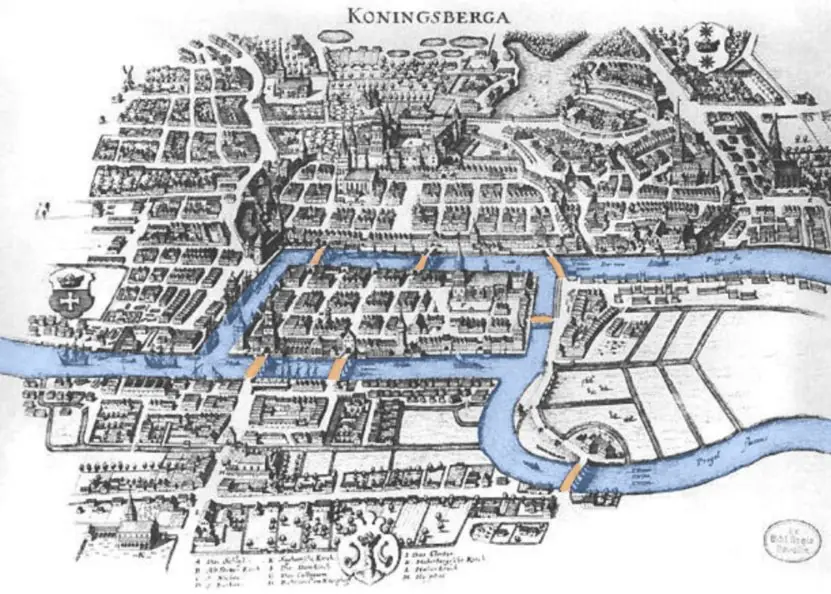
Leonhard Euler turned a puzzle about the bridges of Konigsberg into the first theorem of graph theory. He ignored the shape of the land and kept only four land masses (vertices) and seven bridges (edges).

A walk that uses every bridge exactly once can exist only if zero or two vertices have an odd degree. Plate 5.1 counts the degrees from the bridge list: all four land masses are odd, so no such walk exists.

(a) Konigsberg and its seven bridges (Merian's map, 1652)

(b) Degrees of the four land masses

5.2 Traversal, connectivity and Euler/Hamilton

Breadth-first search (BFS) explores by layers using a queue and finds shortest paths (in edges). Depth-first search (DFS) goes as deep as possible using a stack or recursion; used for cycle detection, topological sort and components.

Both run in O (V + E) with adjacency lists.

Euler circuit (uses every edge exactly once and returns): exists in a connected graph iff every degree is even. Euler path (not returning): exists iff exactly two vertices have odd degree (start and end there).

The Königsberg bridges h a d four odd-degree land masses, so no walk exists.

Hamilton circuit visits every vertex exactly once. There is no simple criterion (the problem is NP-complete). Dirac's sufficient condition: n \geq 3 and deg(v) ≥ \frac{n}{2} for all v.

The travelling salesman problem asks for the cheapest Hamilton circuit; K_{10} has \frac{9 !}{2} = 181,440 distinct circuits.

Euler's formula V - E + F = 2

For a connected graph drawn on a plane without crossings, the number of vertices minus the number of edges plus the number of faces (counting the outside) is always 2. The five regular solids, flattened onto a plane, all obey it.

This fact is what proves that K5 and K3,3 cannot be drawn without crossings. Plate 5.2 checks V - E + F for the five Platonic solids from their vertex, edge and face counts.

(a) Leonhard Euler (1707-1783)

(b) V - E + F for the five regular solids

5.3 Planarity and colouring

A graph is planar if it can be drawn without crossing edges. Euler's formula for a connected planar graph: V - E + F = 2 (F counts the outer face). For simple planar graphs with V \geq 3: E ≤ 3V − 6 (and E ≤ 2V − 4 if bipartite).

K_{5} (10 > 3·5 − 6 = 9) and K₃,₃ (9 > 2·6 − 4 = 8) are not planar, and Kuratowski's theorem says a graph is planar iff it contains no subdivision of K_{5} or K₃,₃.

Colouring. A proper colouring gives adjacent vertices different colours; the chromatic number \chi (G) is the minimum number of colours. \chi (K_{n}) = n ;\ \chi ( \mathrm{even} cycle) = 2 ;\ \chi ( \mathrm{odd} cycle) = 3 ;\ \chi (\mathrm{bipartite}) = 2; four-colour theorem: every planar graph has \chi \leq 4.

Applications: exam timetabling (vertices are exams, edges connect exams that share students, colours are time slots), register allocation, frequency assignment.

Colouring a map

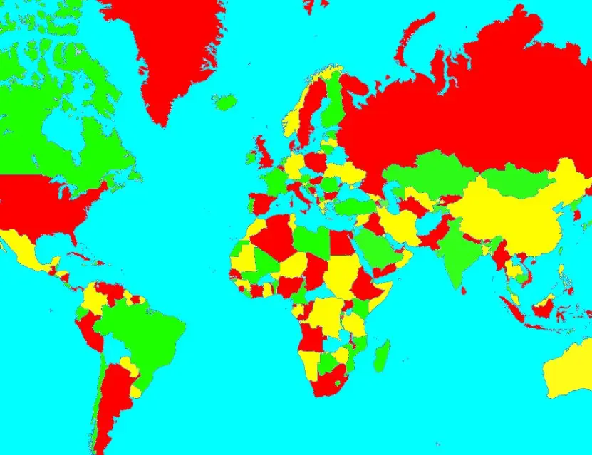
To colour a map, treat each region as a vertex and join two vertices when the regions share a border; neighbouring regions need different colours. The four colour theorem says four colours always suffice for a map on a plane.

A simple greedy rule, giving each region the smallest colour not used by its neighbours, often needs fewer.

Plate 5.3 colours a h u b region ringed by six neighbours: the greedy method uses three colours, and the check confirms no two neighbours share one.

(a) World map in four colours (four colour theorem)

(b) Greedy colouring of a hub with six neighbours

5.4 Weighted graphs: shortest paths and spanning trees

Consider the weighted graph with edges AB 4, AC 2, BC 1, BD 5, CD 8, CE 10, DE 2, DF 6, EF 3.

Dijkstra's algorithm (non-negative weights): keep a tentative distance for each vertex (0 for the source, \infty for the rest); repeatedly fix the closest unfixed vertex and relax the edges out of it.

Spanning tree: a subgraph that is a tree containing all vertices. A connected graph with V vertices has spanning trees of exactly V - 1 edges. A minimum spanning tree (MST) has least total weight.

Kruskal's algorithm: sort edges by weight; add each edge unless it makes a cycle (use union–find). Prim's algorithm: grow a tree from a start vertex, always adding the cheapest edge leaving the tree.

5.5 Trees

A tree is a connected graph with no cycles. Equivalent statements (for n vertices): connected and n - 1 edges; acyclic and n - 1 edges; exactly one path between any two vertices; connected and removing any edge disconnects it.

Every tree with n \geq 2 vertices has at least two leaves (degree-1 vertices).

Rooted trees. Terms: root, parent, child, sibling, leaf, internal node, level (root 0), height (longest root-to-leaf path), subtree. A binary tree has at most two children per node; an m-ary tree at most m.

A full m-ary tree with i internal nodes has n = mi + 1 nodes and l = ( m − 1)i + 1 leaves. A binary tree of height h has at most 2^{h+1} - 1 nodes and at most 2^{h} leaves, so n nodes need height at least \lfloor \log_{2} n \rfloor.

Traversals of a binary tree. Preorder (root, left, right), inorder (left, root, right), postorder (left, right, root), and level order (BFS).

Binary search trees keep left < node < right, so inorder traversal gives sorted order; search, insert and delete take O (\mathrm{height}): O (\log n) if balanced (AVL, red–black), O (n) if skewed.

Heaps and tries are other trees; decision trees show that any comparison sort needs at least \lceil \log_{2} n ! \rceil comparisons (about n \log_{2} n).

Huffman coding builds an optimal prefix code tree by repeatedly merging the two least frequent symbols.

Frequencies a 45 ,\ b 13 ,\ c 12 ,\ d 16 ,\ e 9 ,\ f 5 (total 100): merge f + e = 14; merge c + b = 25; merge 14 + d = 30; merge 25 + 30 = 55; merge a + 55 = 100.

Codes: a = 0 (1 bit), c = 100 ,\ b = 101 ,\ d = 111 ,\ f = 1100 ,\ e = 1101. Average length = 0.45·1 + 0.12·3 + 0.13·3 + 0.16·3 + 0.05·4 + 0.09·4 = 2.24 bits, against 3 bits for a fixed-length code.

5.6 One graph, three answers

The weighted graph of Section 5.4 can be read three ways at once (Figure 5.1).

The red numbers beside each city are the Dijkstra distances from A. The thick teal edges are the minimum spanning tree found by Kruskal and Prim, with total weight 13. The thin grey edges are the ones both algorithms rejected.

Notice that the shortest path to F (A–C–B–D–E–F, length 13) and the spanning tree are different things: the tree connects everyone cheaply, while a shortest path serves one pair of cities.

Think of A as a district office and the other letters as health posts: the spanning tree is the cheapest cable network, Dijkstra tells you the fastest road from the office to each post.

5.7 Eight uses of graphs and trees

1. Maps and navigation. Road networks are weighted graphs, and Dijkstra-type algorithms find the fastest route. A ride-hailing a p p in Kathmandu recomputes shortest paths every few seconds as traffic weights change.
2. Computer networks. Routers form a graph, and protocols such as OSPF run a shortest-path algorithm to choose where each packet goes. A spanning tree protocol on a college switch stops loops from flooding the network.
3. Social networks. People are vertices and friendships are edges. Degrees show who is popular, BFS finds how many steps separate two people, and components show separate communities.
4. Scheduling and timetables. Exams, classes or tasks that clash are joined by edges, and a proper colouring gives the time slots. A campus needing 3 colours has a clash-free exam routine in 3 sessions.
5. Utility networks. A minimum spanning tree gives the cheapest cable, pipe or road layout that links every village or ward. Kruskal's 13-unit answer in Figure 5.1 is a toy version of planning a rural electricity grid.
6. File systems and data structures. Folders form a rooted tree, and search trees and heaps keep data ordered for fast lookup. A binary search tree of 1,000,000 records needs only about 20 comparisons when it is balanced.
7. Compilers and expressions. A parser turns an expression such as (3 + 4) \times 5 into a tree, and postfix traversal gives the order a stack machine evaluates it. Spreadsheet formulas use the same idea.
8. Compression. Huffman coding builds a tree in which frequent symbols get short codes. In the worked example the average falls to 2.24 bits against 3, a saving of about 25 per cent, which is how ZIP and JPEG shrink files.

Formula and fact sheet

• \sum \deg = 2E; K_{n} has \frac{n (n - 1)}{2} edges; K_{m ,\ n} has m n.
• Euler circuit: all degrees even; Euler path: exactly two odd.
• Planar: V - E + F = 2 ;\ E ≤ 3V − 6. K_{5} and K₃,₃ non-planar. Four-colour theorem.
• Tree: connected, acyclic, n - 1 edges. Binary tree of height h: ≤ 2^{h+1} - 1 nodes.
• BFS/DFS O (V + E); Dijkstra O ((V + E) \log V); Kruskal O (E \log E).
• Traversals: pre (root first), in (root middle), post (root last).

Chapter summary

• Graphs are vertices and edges; degree, paths and connectivity answer structural questions, and the handshake lemma constrains degrees.
• Euler's theorem decides Euler circuits by degrees; Hamilton circuits have no simple test.
• Planarity and colouring have formulas and applications in scheduling.
• Dijkstra gives shortest paths and Kruskal/Prim give minimum spanning trees.
• Trees are acyclic connected graphs; traversals, search trees and Huffman codes are their main uses.

Practice

1. A graph has 8 vertices, each of degree 3. How many edges? Does it have an Euler circuit?
2. Draw K_{4} and give its adjacency matrix. How many Hamilton circuits does K_{5} have?
3. Does a graph with degree sequence (2, 2, 4, 4, 2, 2) have an Euler circuit if it is connected? Find |E|.
4. Show that K₃,₃ is not planar using E ≤ 2V − 4.
5. A planar connected graph has 7 vertices and 10 edges. How many faces?
6. Run BFS and DFS on: A: B, D; B: A, C; C: B, D, E; D: A, C; E: C.
7. Apply Dijkstra from S: SA 7, SB 2, BA 3, AC 1, BC 8, CT 2, AT 6. Give the shortest distance to T.
8. Find an MST of the same graph with Kruskal.
9. Write the preorder, inorder and postorder of the tree with root 8, left child 3 (children 1 and 6), right child 10 (right child 14).
10. A full binary tree has 15 leaves. How many internal nodes and total nodes?

Answers and worked solutions

1. 8·3/2 = 12 edges; degrees are odd, so no Euler circuit.

2. Adjacency matrix of K_{4}: 0 on the diagonal, 1 elsewhere. K_{5} Hamilton circuits: \frac{(5 - 1) !}{2} = 12.

3. All degrees even and connected, so yes; sum = 16 \Rightarrow |E| = 8.

4. V = 6 ,\ E = 9; bipartite planar graphs need E ≤ 2V − 4 = 8 ;\ 9 > 8, so not planar.

5. F = 2 - V + E = 2 - 7 + 10 = 5 faces.

6. BFS: A, B, D, C, E. DFS: A, B, C, D, E (from A visit B; B visits C; C visits D (D's neighbour A visited), then E).

7. S = 0 ;\ B = 2 ;\ A = \min (7 ,\ 2 + 3) = 5 ;\ C = \min (2 + 8 ,\ 5 + 1) = 6 ;\ T = \min (5 + 6 ,\ 6 + 2) = 8 (path S–B–A–C–T).

8. Sorted: AC 1, SB 2, CT 2, BA 3, AT 6, SA 7, BC 8. Take AC, SB, CT, BA (joins {S,B} with {A,C,T}) = 4 edges for 5 vertices. MST weight = 1 + 2 + 2 + 3 = 8.

9. Preorder 8, 3, 1, 6, 10, 14. Inorder 1, 3, 6, 8, 10, 14 (sorted, since it is a BST). Postorder 1, 6, 3, 14, 10, 8.

10. l = i + 1 for a full binary tree, so i = 14; total nodes = 14 + 15 = 29.

Model answers: medium (5 marks) and long (10 marks) questions

Q1 (5 marks). Explain Kruskal's algorithm and find a minimum spanning tree of the graph in Figure 5.1.

Introduction. A spanning tree of a connected graph with V vertices is a subgraph with V - 1 edges that connects all vertices without a cycle. A minimum spanning tree (MST) is the one with the smallest total weight. Kruskal's algorithm builds it greedily.

Algorithm.

1. Sort all edges by weight.
2. Take the next smallest edge.
3. Add it if it joins two different components; skip it if it would form a cycle (checked with union–find).
4. Stop when V - 1 edges are chosen.

Solution. Sorted edges: BC 1, AC 2, DE 2, EF 3, AB 4, BD 5, DF 6, CD 8, CE 10. Take BC, AC, DE, EF. AB (4) is skipped because A and B are already joined through C. BD (5) joins {A, B, C} to {D, E, F}, so it is taken. That is 5 = 6 - 1 edges, so we stop.

Step	Edge	Weight	Decision
1	BC	1	take
2	AC	2	take
3	DE	2	take
4	EF	3	take
5	AB	4	skip (cycle A - B - C)
6	BD	5	take

Conclusion. MST weight = 1 + 2 + 2 + 3 + 5 = 13. Prim's algorithm starting at A gives the same total. Sorting makes Kruskal run in O (E \log E).

Q2 (10 marks). Describe Dijkstra's algorithm, apply it to the graph of Figure 5.1 from A, and explain how it differs from BFS and from a minimum spanning tree.

Introduction. The shortest-path problem asks for the least-weight route from a source to every other vertex of a weighted graph. Dijkstra's algorithm solves it when all weights are non-negative.

Algorithm.

1. Set the distance of the source to 0 and all others to infinity.
2. Pick the unfixed vertex with the smallest tentative distance and fix it.
3. For each neighbour, relax the edge: if d (u) + w < d (v), replace d (v).
4. Repeat until every vertex is fixed.

*Working from A . \ast

Fixed vertex	B	C	D	E	F
A (0)	4	2	\infty	\infty	\infty
C (2)	3	–	10	12	\infty
B (3)	–	–	8	12	\infty
D (8)	–	–	–	10	14
E (10)	–	–	–	–	13
F (13)	–	–	–	–	–

Result. Distances from A: B 3, C 2, D 8, E 10, F 13. The shortest path to F is A \to C \to B \to D \to E \to F, with length 2 + 1 + 5 + 2 + 3 = 13.

Differences.

5. BFS counts edges, not weights, so it finds the path with the fewest hops (A to F is 3 hops via C, D) even when it is heavier. Dijkstra uses weights.
6. MST connects all vertices at the least total cost (13 here) and has no source. A tree path inside the MST can be longer than the shortest path.
7. Negative weights break Dijkstra because a fixed vertex could later be improved; Bellman–Ford is used instead.
8. Cost. With a priority queue Dijkstra runs in O ((V + E) \log V).

Feature	BFS	Dijkstra	MST (Kruskal/Prim)
Uses weights	no	yes	yes
Goal	fewest edges	least path weight	least total weight
Needs a source	yes	yes	no
Output	layers	distance table	V - 1 edges

Conclusion. Dijkstra fixes vertices in increasing order of distance and relaxes edges, giving all shortest paths from one source. It answers a different question from BFS or an MST, even on the same graph.