Unit 3 · 5 teaching hours · 21 min read
Numerical Differentiation and Integration
What the syllabus asks for 5
- Numerical differentiation
- Numerical integration: Newton–Cotes rules
- Romberg integration
- Numerical double integration
- Seeing the ideas: areas under curves, Romberg's table and the error of a derivative
A speedometer log gives positions every few seconds: what is the speed? A sensor gives readings: what is the total?
Differentiation and integration of tabulated data, or of functions with no elementary antiderivative such as e^{- x^{2}} and \frac{1}{\ln x}, must be done numerically.
The formulas here come from differentiating or integrating the interpolating polynomials of Unit 2.
- Finite-difference formulas for derivatives and their errors; Newton's differentiation formulas.
- Newton–Cotes integration: trapezoidal, Simpson's \frac{1}{3} and \frac{3}{8} rules, composite versions and error behaviour.
- Romberg integration and numerical double integration.
3.1 Numerical differentiation
From f (x + h) = f (x) + h f' (x) + \left( \frac{h^{2}}{2} \right) f'' (x) + \ldots we get three basic formulas:
| Formula | Expression | Error order |
|---|---|---|
| Forward difference | f' (x) \approx \frac{f (x + h) - f (x)}{h} | O (h) |
| Backward difference | f' (x) \approx \frac{f (x) - f (x - h)}{h} | O (h) |
| Central difference | f' (x) \approx \frac{f (x + h) - f (x - h)}{2 h} | O (h^{2}) |
| Central, second derivative | f'' (x) \approx \frac{f (x + h) - 2 f (x) + f (x - h)}{h^{2}} | O (h^{2}) |
The central formula is better because the first error term cancels. Halving h should cut the forward error by 2 and the central error by 4.
| h | forward \frac{f (x + h) - f (x)}{h} | error | central \frac{f (x + h) - f (x - h)}{2 h} | error |
|---|---|---|---|---|
| 0.1 | 2.858842 | 0.140560 | 2.722815 | 0.0045327 |
| 0.01 | 2.731919 | 0.013637 | 2.718327 | 0.0000453 |
| 0.001 | 2.719641 | 0.001360 | 2.718282 | 0.0000005 |
Each tenfold reduction of h reduces the forward error about tenfold and the central error about a hundredfold, exactly as the orders say.
(The backward formula with h = 0.1 gives 2.586787, an error of the opposite sign to the forward one.) If h is made too small, round-off error (subtracting nearly equal numbers) eventually dominates: there is an optimal h (roughly 10^{-8} for the forward formula and 10^{-5} for the central formula in double precision), below which the total error grows again.
Newton's differentiation formulas (tabulated, equally spaced data)
Differentiating Newton's forward formula (Unit 2) with respect to x at x = x_{0} (u = 0) gives
(At the end of a table use the backward versions with ∇ and plus signs.)
| x | y = \ln x | \Delta y | \Delta^{2} y | \Delta^{3} y | \Delta^{4} y |
|---|---|---|---|---|---|
| 1.0 | 0.000000 | 0.095310 | -0.008299 | 0.001330 | -0.000296 |
| 1.1 | 0.095310 | 0.087011 | -0.006969 | 0.001034 | |
| 1.2 | 0.182322 | 0.080043 | -0.005935 | | |
| 1.3 | 0.262364 | 0.074108 | | | |
| 1.4 | 0.336472 | | | | |
With h = 0.1, using more terms improves the answer: one term gives 0.953102, two terms 0.994596, three 0.999030, and four terms f' (1.0) \approx 0.999770 (error 0.000230).
The second derivative from the formula is f'' (1.0) \approx - 0.990045 (true −1; the error is larger because a second derivative loses accuracy).
For an interior point use central formulas instead. At x = 1.2: f' \approx \frac{\ln 1.3 - \ln 1.1}{0.2} = 0.835270 (true 1 / 1.2 = 0.833333) and f'' \approx \frac{\ln 1.1 - 2 \ln 1.2 + \ln 1.3}{0.01} = - 0.696867 (true - 1 / 1.2^{2} = - 0.694444).
Maxima and minima of a tabulated function. Differentiate Newton's formula, set \frac{d y}{d u} = 0, solve for u (usually a quadratic) and convert to x = x_{0} + h u; use the second derivative to classify.
3.2 Numerical integration: Newton–Cotes rules
To compute I = \int_{a}^{b} f (x) \,d x, divide [a ,\ b] into n equal strips of width h = \frac{b - a}{n} ,\ x_{i} = a + ih, y_{i} = f (x_{i}), replace f on groups of strips by an interpolating polynomial, and integrate that exactly.
| Rule | Polynomial | Formula (composite) | n must be | Error |
|---|---|---|---|---|
| Trapezoidal | line (1 strip) | \left( \frac{h}{2} \right) [y_{0} + 2 (y_{1} + \ldots + y_{n-1}) + y_{n}] | any | - \frac{(b - a) h^{2} f'' (\xi)}{12} ,\ O (h^{2}) |
| Simpson's \frac{1}{3} | parabola (2 strips) | \left( \frac{h}{3} \right) [y_{0} + 4 (y_{1} + y_{3} + \ldots) + 2 (y_{2} + y_{4} + \ldots) + y_{n}] | even | - \frac{(b - a) h^{4} f'''' (\xi)}{180} ,\ O (h^{4}) |
| Simpson's \frac{3}{8} | cubic (3 strips) | \left( \frac{3 h}{8} \right) [y_{0} + 3 (y_{1} + y_{2} + y_{4} + y_{5} + \ldots) + 2 (y_{3} + y_{6} + \ldots) + y_{n}] | multiple of 3 | - \frac{(b - a) h^{4} f'''' (\xi)}{80} ,\ O (h^{4}) |
Simpson's \frac{1}{3} rule is exact for polynomials up to degree 3 (not just 2) because the odd error term vanishes; the \frac{3}{8} rule is also exact to degree 3. The trapezoidal rule is exact only for lines.
Function values:
| i | x_{i} | f (x_{i}) = \frac{1}{(1 + x_{i}^{2})} |
|---|---|---|
| 0 | \frac{0}{6} | 1.000000 |
| 1 | \frac{1}{6} | 0.972973 |
| 2 | \frac{2}{6} | 0.900000 |
| 3 | \frac{3}{6} | 0.800000 |
| 4 | \frac{4}{6} | 0.692308 |
| 5 | \frac{5}{6} | 0.590164 |
| 6 | \frac{6}{6} | 0.500000 |
Trapezoidal. \frac{h}{2} \times [y_{0} + y_{6} + 2 (y_{1} + \ldots + y_{5})] = \left( \frac{1}{6} \right) \left[ \frac{1.000000 + 0.500000}{2} + \sum y_{1} \ldots y_{5} \right]: the bracketed sum is 4.705445, so I ≈ 0.784241, error 0.001157.
Simpson's \frac{1}{3}. \left( \frac{h}{3} \right) [y_{0} + y_{6} + 4 (y_{1} + y_{3} + y_{5}) + 2 (y_{2} + y_{4})] = \left( \frac{1}{18} \right) [1.500000 + 4 (2.363137) + 2 (1.592308)] = \left( \frac{1}{18} \right) (14.137163) = 0.785398, error 0.0000002.
Simpson's \frac{3}{8}. \left( \frac{3 h}{8} \right) [y_{0} + y_{6} + 3 (y_{1} + y_{2} + y_{4} + y_{5}) + 2 y_{3}] gives 0.785396, error 0.0000023.
Simpson's rules are about a thousand times more accurate than the trapezoidal rule with the same data. (All three results were checked against SciPy's quad.)
Convergence as n grows
| n | trapezoid | error | Simpson \frac{1}{3} | error |
|---|---|---|---|---|
| 2 | 0.775000 | 1.04e-02 | 0.783333 | 2.06e-03 |
| 4 | 0.782794 | 2.60e-03 | 0.785392 | 6.01e-06 |
| 8 | 0.784747 | 6.51e-04 | 0.785398 | 3.78e-08 |
| 16 | 0.785235 | 1.63e-04 | 0.785398 | 5.91e-10 |
Each doubling of n divides the trapezoidal error by about 4 (order h^{2}) and the Simpson error by about 16 (order h^{4}), as the error terms predict.
Choosing a rule: use Simpson's \frac{1}{3} when the number of strips is even, the \frac{3}{8} rule when it is a multiple of 3, or combine them (\frac{3}{8} on three strips plus \frac{1}{3} on the rest) for odd n.
Use the trapezoidal rule for rough work, noisy data, or periodic functions integrated over a full period.
3.3 Romberg integration
Richardson extrapolation combines two estimates with step h and \frac{h}{2} to cancel the leading error term. Applied repeatedly to trapezoidal values, it gives the Romberg table:
R ( k, 0) = trapezoidal rule with 2^{k} strips; R (k ,\ j) = R (k ,\ j - 1) + \frac{R (k ,\ j - 1) - R (k - 1 ,\ j - 1)}{4^{j} - 1}.
Column 1 is Simpson's \frac{1}{3} rule, column 2 is Boole's rule, and each further column cancels the next error power (h^{2} ,\ h^{4} ,\ h^{6} ,\ \ldots).
| h | R (k ,\ 0) trapezoid | R (k ,\ 1) | R (k ,\ 2) | R (k ,\ 3) | R (k ,\ 4) |
|---|---|---|---|---|---|
| 1 | 0.75000000 | | | | |
| \frac{1}{2} | 0.77500000 | 0.78333333 | | | |
| \frac{1}{4} | 0.78279412 | 0.78539216 | 0.78552941 | | |
| \frac{1}{8} | 0.78474712 | 0.78539813 | 0.78539852 | 0.78539645 | |
| \frac{1}{16} | 0.78523540 | 0.78539816 | 0.78539817 | 0.78539816 | 0.78539817 |
The best estimate R (4 ,\ 4) = 0.78539817 differs from \frac{\pi}{4} = 0.78539816 by only 2.92e-09 (using just 17 function values).
Note that the extrapolated values do not improve in every single entry: R (3 ,\ 3) = 0.78539645 has error 1.72e-06, which is larger than R (3 ,\ 2).
The table improves in the limit; the stopping rule is \mid R (k ,\ k) - R ( k - 1 ,\ k − 1)| < ε.
3.4 Numerical double integration
For I = \int_{a}^{b} \int_{c}^{d} f (x ,\ y) \,d y \,d x, apply a one-dimensional rule in each direction. With a grid h_{x} \times k_{y}, the composite rule is a double sum of the weights times function values.
For Simpson's \frac{1}{3} with two strips in each direction the weights form the grid
| y_{0} | y_{1} | y_{2} | |
|---|---|---|---|
| x_{0} | 1 | 4 | 1 |
| x_{1} | 4 | 16 | 4 |
| x_{2} | 1 | 4 | 1 |
and I \approx \left( \frac{h_{x} k}{9} \right) \sum w_{ij} f (x_{i} ,\ y_{j}). For the trapezoidal rule the weights are \frac{1}{4} ,\ \frac{1}{2} ,\ \frac{1}{4} products and I \approx h_{x} k \sum w_{ij} f.
The exact value is 3 \ln 3 - 4 \ln 2 = 0.523248.
| f (x ,\ y) = \frac{1}{x + y} | y = 1 | y = 1.5 | y = 2 |
|---|---|---|---|
| x = 0 | 1.000000 | 0.666667 | 0.500000 |
| x = 0.5 | 0.666667 | 0.500000 | 0.400000 |
| x = 1.0 | 0.500000 | 0.400000 | 0.333333 |
Simpson (weights 1, 4, 1): I \approx (0.5 \times 0.5 / 9) \times \sum = 0.524074, error 0.000826. Trapezoidal: 0.537500, error 0.014252. Even with only nine points Simpson is accurate to 3 decimals.
A smaller step or a Romberg refinement in each direction would improve both.
3.5 Seeing the ideas: areas under curves, Romberg's table and the error of a derivative
Before computers, engineers measured the area of an irregular shape with a mechanical planimeter, a hand-driven integrator. Numerical integration does the same job with arithmetic.
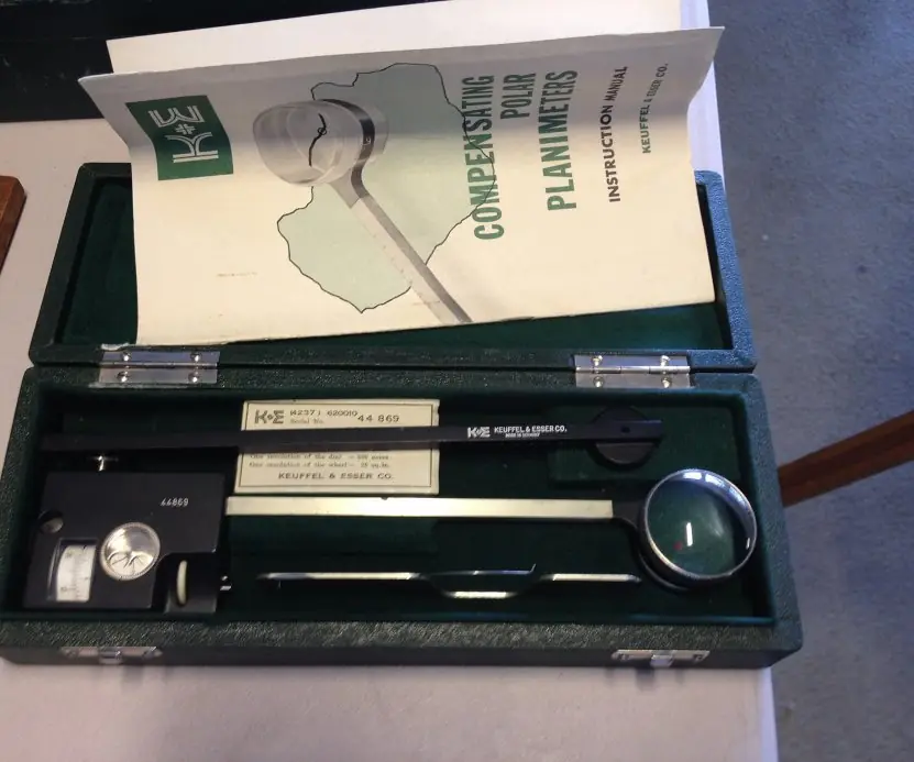


3.5.1 Eight uses of numerical integration and differentiation
- Area and volume of irregular shapes. Land surveyors in Nepal measure a field boundary at fixed intervals, and Simpson's rule gives the area. The same idea gives the volume of earth to cut for a road. No formula for the shape is needed.
- Water in a river or reservoir. Flow is measured at several depths and widths. Integrating velocity times area gives the discharge in cubic metres per second. Hydropower planning for rivers such as the Kaligandaki depends on this.
- Distance from speed. A vehicle log gives speed at each minute, and integration adds it into distance travelled. Fitness watches and GPS units do this all day. The trapezoidal rule is enough for such data.
- Work, energy and charge. The work done by a variable force and the charge stored from a varying current are integrals of measured tables. Engineers use numerical integration when the signal is only a list of readings. Oscilloscopes do this inside.
- Probability and statistics. The normal distribution has no closed-form integral, so the tables in textbooks were made numerically. Computers still integrate to find probabilities and p-values. This is the root of all statistical software.
- Rates of change from data. Speed from positions, growth rate from population counts and slope of a sensor curve are numerical derivatives. A central difference gives a good estimate from two neighbouring readings. It is used in control systems and tracking.
- Error control by Romberg and step halving. Halving the step and extrapolating improves the answer without a formula for the error. We know how many digits to trust. This makes numerical results reliable.
- Solving differential equations. Euler and Runge-Kutta methods in the next unit are built from the same ideas of stepping and averaging slopes. Understanding integration therefore opens the way to simulation. Weather and engineering models rest on it.

Formula and fact sheet
- Forward/backward: O (h); central: \frac{f (x + h) - f (x - h)}{2 h} ,\ O (h^{2}) ;\ f'' \approx \frac{f (x + h) - 2 f (x) + f (x - h)}{h^{2}}.
- Trapezoidal: \left( \frac{h}{2} \right) \left[ y_{0} + 2 \sum y_{i} + y_{n} \right]. Simpson \frac{1}{3} ( n even): \left( \frac{h}{3} \right) \left[ y_{0} + 4 \sum \mathrm{odd} + 2 \sum \mathrm{even} + y_{n} \right]. Simpson \frac{3}{8} ( n multiple of 3): \left( \frac{3 h}{8} \right) [\ldots].
- Error orders: trapezoid h^{2}, Simpson h^{4}.
- Romberg: R (k ,\ j) = R (k ,\ j - 1) + \frac{R (k ,\ j - 1) - R (k - 1 ,\ j - 1)}{4^{j} - 1}.
- Double integral: weighted sum with product weights.
Chapter summary
- Derivatives come from differentiating interpolation polynomials; central differences are second-order and best; too small an h lets round-off dominate.
- Newton–Cotes rules integrate interpolating polynomials; Simpson's rules beat the trapezoidal rule at the same cost.
- Romberg extrapolation turns cheap trapezoidal values into a high-order estimate.
- Double integrals reuse the one-dimensional rules with product weights.
Practice
- Derive the forward-difference formula for f' (x) from Taylor's series and state its order.
- For f (x) = e^{x} at x = 1 with h = 0.1, compute forward and central estimates and their errors.
- Estimate f' (1.0) and f'' (1.0) for \ln x from the difference table, using Newton's forward formulas.
- Evaluate \frac{\int_{0}^{1} d x}{(1 + x^{2})} with n = 6 by the trapezoidal, Simpson \frac{1}{3} and Simpson \frac{3}{8} rules.
- Why must n be even for Simpson's \frac{1}{3} rule and a multiple of 3 for the \frac{3}{8} rule?
- How many times smaller is the error expected after halving h for the trapezoidal rule and for Simpson's rule?
- Build a Romberg table with four trapezoidal estimates and extrapolate.
- Estimate \frac{\int_{0}^{1} \int_{1}^{2} d y d x}{x + y} with Simpson's rule, h = k = 0.5, and compare it with the exact value.
- State two reasons why a very small h does not give a better numerical derivative.
Answers and worked solutions
1. f (x + h) = f (x) + h f' (x) + \left( \frac{h^{2}}{2} \right) f'' (\xi). Rearranging, f' (x) = \frac{f (x + h) - f (x)}{h} - \left( \frac{h}{2} \right) f'' (\xi). The truncation error is proportional to h: first order, O (h).
2. The table in Section 3.1 gives forward 2.858842 (error 0.140560) and central 2.722815 (error 0.0045327) for h = 0.1.
3. From the difference table: f' (1.0) \approx 0.999770 and f'' (1.0) \approx - 0.990045 (true values 1 and −1).
4. Trapezoidal 0.784241; Simpson \frac{1}{3} 0.785398; Simpson \frac{3}{8} 0.785396; true 0.785398.
5. Simpson's \frac{1}{3} fits a parabola through three points, covering two strips, so strips must be paired. The \frac{3}{8} rule fits a cubic through four points, covering three strips.
6. Trapezoid error ∝ h^{2}, so halving h divides it by about 4; Simpson ∝ h^{4}, so by about 16 (compare the convergence table in Section 3.2).
7. See the Romberg table in Section 3.3: the extrapolated R (4 ,\ 4) = 0.78539817.
8. Simpson: 0.524074; exact: 0.523248; error 0.000826 (the trapezoidal rule gives 0.537500).
9. Truncation error falls with h, but round-off grows because f (x + h) - f (x) subtracts nearly equal numbers, then is divided by a tiny h; and measured data carry noise which is amplified by \frac{1}{h}. Beyond an optimal h the total error increases.
Model answers: medium (5 marks) and long (10 marks) questions
Q1 (5 marks). Evaluate the integral of \sin x from 0 to pi using the trapezoidal rule and Simpson's one-third rule with four strips. Compare with the exact value.
Data. h = pi/4 = 0.785398; the ordinates are y0 = 0, y1 = 0.70711, y2 = 1, y3 = 0.70711, y4 = 0.
Trapezoidal rule. T = \left( \frac{h}{2} \right) [ y 0 + 2 ( y 1 + y2 + y3) + y4] = 0.392699 x [0 + 2 (2.41421) + 0] = 1.89612.
Simpson's rule. S = \left( \frac{h}{3} \right) [ y 0 + 4 ( y 1 + y3) + 2 y2 + y4] = 0.261799 x [0 + 4 (1.41421) + 2 + 0] = 0.261799 x 7.65685 = 2.00456.
| Rule | Value | Exact | Error |
|---|---|---|---|
| Trapezoidal | 1.89612 | 2 | 0.10388 |
| Simpson \frac{1}{3} | 2.00456 | 2 | -0.00456 |
Simpson is more than twenty times more accurate for the same ordinates (Figure 3.1) because it fits parabolas, not straight lines; its error is of order h^{4}, against h^{2} for the trapezoidal rule.
Condition Simpson's \frac{1}{3} rule needs an even number of strips.
Conclusion use Simpson's rule for smooth functions.
Q2 (5 marks). Estimate the derivative of e^{x} at x = 1 by the forward and central difference formulas with h = 0.1 and h = 0.05, and comment on the errors.
Formulas. Forward: f' (x) is about \frac{f (x + h) - f (x)}{h}, error O (h). Central: f' (x) is about \frac{f (x + h) - f (x - h)}{2 h}, error O (h^{2}). Exact value e = 2.71828.
| h | Forward | Error | Central | Error |
|---|---|---|---|---|
| 0.1 | 2.85884 | 0.14056 | 2.72281 | 0.00453 |
| 0.05 | 2.78739 | 0.06910 | 2.71941 | 0.00113 |
Halving h halves the forward error (0.14056 to 0.06910) but divides the central error by four (0.00453 to 0.00113), as the orders predict (Figure 3.3).
Warning making h extremely small loses accuracy through rounding error in the subtraction.
Conclusion prefer the central formula when values on both sides are available.
Q3 (10 marks). Explain the Newton-Cotes rules and Romberg integration. Apply Romberg's method to the integral of e^{x} on [0, 1].
Introduction. When an integral has no closed form or the integrand is only a table, we replace f by an interpolating polynomial and integrate that (Plate 3.1 shows an older mechanical way). The resulting formulas are the Newton-Cotes rules.
Rules. (1) Trapezoidal: integral is about \left( \frac{h}{2} \right) [y 0 + 2 (y 1 + \ldots + y (n - 1)) + y n], error - \frac{(b - a) h^{2} f''}{12}.
(2) Simpson \frac{1}{3}: \left( \frac{h}{3} \right) [y 0 + 4 (\mathrm{odd}) + 2 (\mathrm{even}) + y n] ,\ n even, error - \frac{(b - a) h^{4} f''''}{180}.
(3) Simpson \frac{3}{8}: \left( \frac{3 h}{8} \right) [ y 0 + 3y1 + 3y2 + 2y3 + \ldots + y n ] ,\ n a multiple of 3, same order. Figure 3.1 compares the first two.
Romberg. The trapezoidal error expands in even powers of h, so Richardson extrapolation removes them one by one: R (i ,\ j) = R (i ,\ j - 1) + \frac{R (i ,\ j - 1) - R (i - 1 ,\ j - 1)}{4^{j} - 1}.
Start with trapezoid values for h = 1 ,\ \frac{1}{2} ,\ \frac{1}{4}: T (1) = 0.5 (1 + 2.718282) = 1.859141 ;\ T (2) = 1.753931 ;\ T (4) = 1.727222.
First extrapolation: R (2 ,\ 1) = 1.753931 + \frac{1.753931 - 1.859141}{3} = 1.718861; R (3 ,\ 1) = 1.727222 + \frac{1.727222 - 1.753931}{3} = 1.718319.
Second: R (3 ,\ 2) = 1.718319 + \frac{1.718319 - 1.718861}{15} = 1.718283, against the exact e - 1 = 1.718282 (Figure 3.2).
| Rule | Order of error | Needs | Best for |
|---|---|---|---|
| Trapezoidal | h^{2} | any n | rough data, periodic functions |
| Simpson \frac{1}{3} | h^{4} | even n | smooth functions |
| Simpson \frac{3}{8} | h^{4} | n multiple of 3 | odd strips |
| Romberg | h^{2} ,\ h^{4} ,\ h^{6} \ldots | halving h | high accuracy by reuse |
Conclusion. Romberg integration reaches six correct decimals from only four function evaluations beyond the trapezoid starts, and the difference between successive entries gives a built-in error estimate.
Use Simpson for a quick answer and Romberg when high accuracy is required.