Microservices, Kubernetes, Autoscaling and Queueing Theory

Once capacity is elastic, the application must be built to use it.

Large systems are therefore split into small, independently deployed services, packaged as containers and run by an orchestrator that restarts failures and adds replicas when load rises.

Whether those replicas arrive in time, and how long requests wait while they do, is not guesswork: it follows from a scaling formula and from queueing theory. This unit covers both the architecture and the arithmetic.

5.1 Monolith to microservices

A monolith is one deployable unit: simple to build, test and debug, but it must be scaled, released and failed as a whole.

Microservices divide the system into small services, each owning its data and a single business capability (orders, payments, catalogue), communicating through APIs or events.

Benefits: independent deployment and scaling, technology freedom, fault isolation, team autonomy.

Costs: network calls replace function calls (latency, partial failure), data consistency across services needs patterns such as the saga (a sequence of local transactions with compensating actions) rather than one ACID transaction, and operational complexity rises sharply (service discovery, tracing, versioning).

A well-factored monolith is often the right start for a small team.

Resilience patterns: timeouts and retries with exponential backoff and jitter, circuit breakers (stop calling a failing dependency to let it recover), bulkheads (separate resource pools so one slow dependency cannot exhaust all threads), an API gateway at the edge and a service mesh for uniform security and telemetry between services.

Observability rests on logs, metrics and distributed traces tied together by a correlation ID.

5.2 Kubernetes architecture

Kubernetes (K8s) is the standard open-source container orchestrator. A cluster has a control plane and a set of worker nodes.

• kube-apiserver: the front door; every client and component talks to it through a REST API.
• etcd: the consistent key-value store (Raft-based) holding all cluster state.
• kube-scheduler: assigns unscheduled Pods to nodes by resource requests, affinity, taints and tolerations.
• kube-controller-manager: runs control loops (Deployment, ReplicaSet, Node, and others).
• cloud-controller-manager: integrates with the provider (load balancers, volumes).
• On each node: kubelet (runs Pods and reports status), kube-proxy (Service networking rules) and a container runtime (containerd or CRI-O).

Core objects: a Pod is the smallest unit, one or more containers sharing network and storage; a ReplicaSet keeps a number of Pod copies running; a Deployment manages ReplicaSets and rolling updates; a Service gives a stable virtual IP and DNS name to a changing set of Pods; an Ingress routes external HTTP traffic; ConfigMap and Secret inject configuration; a StatefulSet gives stable identity and storage to stateful workloads; a DaemonSet runs one Pod per node.

5.3 Horizontal Pod Autoscaler

The HPA adjusts the replica count of a Deployment from observed metrics (CPU, memory, or custom metrics). For a target value per Pod, the controller computes:

Scale-down additionally uses a stabilization window (default 300 seconds), taking the highest recommendation in the window to avoid flapping; scale-up is faster by default.

The program traces four evaluations for a target average CPU of 60% with bounds 2 to 10 replicas.

target, min_r, max_r = 60, 2, 10
steps = [(4, 90), (6, 30), (3, 63), (3, 300)]
for i, (cur, metric) in enumerate(steps, 1):
    note = ""
    if abs(metric / target - 1) <= 0.10:
        want = cur
        note = " (within 10% tolerance)"
    else:
        want = -(-cur * metric // target)
        if want > max_r:
            note = f", capped at {max_r}"
    print(f"step {i}: {cur} replicas, metric {metric}% vs target {target}% -> desired {want}{note}")

step 1: 4 replicas, metric 90% vs target 60% -> desired 6
step 2: 6 replicas, metric 30% vs target 60% -> desired 3
step 3: 3 replicas, metric 63% vs target 60% -> desired 3 (within 10% tolerance)
step 4: 3 replicas, metric 300% vs target 60% -> desired 15, capped at 10

Step 1: 4 × 90 ÷ 60 = 6, so the HPA scales out to 6. Step 2: at 6 replicas and 30% load, 6 × 30 ÷ 60 = 3 (scale-in, subject to the stabilization window).

Step 3 shows the tolerance: 63% is only 5% above target, so no change, although the raw formula would give ⌈3 × 63 ÷ 60⌉ = 4 replicas and cause constant small changes. Step 4: a spike to 300% asks for 15, but the maximum of 10 caps it.

5.4 Little's Law and the M/M/1 queue

Little's Law relates the three quantities of any stable system: L = λ × W, where L is the average number of items in the system, λ the average arrival rate and W the average time each item spends in the system.

It needs no assumptions about the distribution of arrivals or service times, only stability.

The M/M/1 queue models one server with Poisson arrivals (rate λ) and exponential service times (rate μ). Utilisation is ρ = λ ÷ μ, and for ρ < 1:

• average number in system L = ρ ÷ (1 − ρ);
• average number waiting Lq = ρ² ÷ (1 − ρ);
• average time in system W = 1 ÷ (μ − λ);
• average waiting time Wq = ρ × W.

lam, mu = 80, 100                       # requests per second arriving, capacity of one worker
rho = lam / mu
L = rho / (1 - rho)
Lq = rho * rho / (1 - rho)
W = 1 / (mu - lam)
Wq = rho * W
print(f"rho {rho:.3f}, L {L:.3f}, Lq {Lq:.3f}, W {W * 1000:.1f} ms, Wq {Wq * 1000:.1f} ms")
print(f"Little check: lambda*W = {lam * W:.3f}")

rho 0.800, L 4.000, Lq 3.200, W 50.0 ms, Wq 40.0 ms
Little check: lambda*W = 4.000

A worker running at 80% utilisation holds four requests on average, with a mean response time of 50 ms of which 40 ms is waiting; the service time alone is 10 ms.

The Little check confirms λ × W = 80 × 0.05 = 4 = L. The curve is nonlinear: raising arrivals to 95 per second (ρ = 0.95) gives L = 19 and W = 200 ms, four times slower for a 19% increase in load.

This is why autoscalers target utilisation of 50% to 70%, not 95%.

5.5 Serverless and concurrency

In Function as a Service, a platform starts a function instance per concurrent request (reusing warm instances), scales to zero when idle, and bills per request and per millisecond of execution.

A cold start is the delay to create a new execution environment (runtime start, code load, initialisation), ranging from tens of milliseconds to seconds depending on language, package size and VPC attachment.

Mitigations include smaller packages, provisioned concurrency and lighter runtimes. Little's Law gives the required concurrency directly: concurrency = arrival rate × duration.

rate, dur, limit = 500, 0.2, 1000
conc = rate * dur
print(f"concurrency needed {round(conc)} ({rate} req/s x {dur} s)")
print(f"utilisation of {limit} limit: {conc / limit * 100:.1f}%")

concurrency needed 100 (500 req/s x 0.2 s)
utilisation of 1000 limit: 10.0%

At 500 requests per second with a 200 ms duration the platform must run 100 instances at once, 10% of a 1,000 default account concurrency limit. Cutting duration to 100 ms halves it.

Providers throttle requests above the limit, and the bill is proportional to total execution time, so optimising function duration cuts both cost and concurrency.

5.6 Seeing the ideas: the cluster, the autoscaler, the monolith and the queue

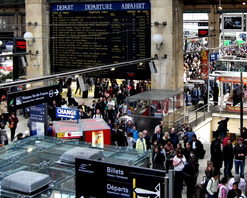
Queueing theory looks abstract until you stand in a line. Plate 5.1 sets a real ticket queue beside the M/M/1 curve that predicts what happens to waiting time as a server gets busier.

(a) Ticket queue at a station

(b) Requests in system versus utilisation

5.6.1 Eight benefits of Kubernetes for cloud applications

1. Self-healing. If a container or a node fails, Kubernetes starts replacements automatically because the observed state no longer matches the declared state. A payment service stays up without a person watching it at night. Health checks also restart containers that hang.
2. Automatic scaling. The Horizontal Pod Autoscaler adds Pods when load rises and removes them when it falls. A ticket-booking site for a festival can grow within minutes. Nodes can be added by a cluster autoscaler as well.
3. Rolling updates and rollbacks. A Deployment replaces old Pods with new ones gradually, so users see no downtime. If the new version fails its checks, one command returns to the old version. Releases become routine instead of risky.
4. Service discovery and load balancing. A Service gives a stable name and address to a changing set of Pods. Other services call it by name and traffic is spread across the healthy Pods. Developers do not track individual IP addresses.
5. Declarative configuration. The whole system is described in YAML files that can be stored in Git and reviewed. The same files rebuild the system in another region. This is the idea of infrastructure as code.
6. Efficient resource use. The scheduler packs Pods onto nodes by their CPU and memory requests, so servers are well filled. Fewer machines are needed for the same work. Namespaces and quotas stop one team from taking everything.
7. Portability. The same manifests run on any major cloud and on a college's own servers. A company can move from one provider to another with much less rework. This reduces vendor lock-in.
8. Rich ecosystem. Tools for monitoring, logging, service mesh, secrets and CI/CD plug into Kubernetes. Skills learnt for one project apply to many employers. Open standards keep the knowledge useful for years.

(a) Turnstiles: open more gates when the queue grows

(b) Autoscaler with and without a cool-down

5.7 Summary and exercises

Microservices trade simplicity for independence; Kubernetes reconciles desired and observed state; the HPA scales replicas by ⌈current × metric ÷ target⌉ within tolerance and bounds; Little's Law and M/M/1 show why queues explode near full utilisation, and give serverless concurrency directly.

1. List the control-plane components of Kubernetes and the role of each.
2. Apply the HPA formula: 5 replicas, CPU 84%, target 70%, bounds 2 to 12. What is the outcome? What if CPU is 74%?
3. Explain why the HPA has a tolerance and a scale-down stabilization window.
4. For λ = 45 req/s and μ = 50 req/s compute ρ, L and W for M/M/1.
5. A function runs 300 ms at 200 invocations per second. What concurrency is needed?
6. Give two advantages and two disadvantages of microservices for a five-person team.

Model answers: medium (5 marks) and long (10 marks) questions

Q1 (5 marks). Compare monolithic and microservice architectures.

Introduction. A monolith is one deployable unit; microservices split the system into small services that each own one business capability and their data (Figure 5.3).

Point	Monolith	Microservices
Deployment	One unit, whole release	Each service separately
Scaling	Whole application	Only the busy service
Fault isolation	One bug can stop all	Failure contained
Technology	One stack	Different stack per service
Data	One shared database	Database per service
Complexity	Simple to build and debug	Network calls, distributed tracing
Best for	Small teams, early stage	Large teams, fast-changing systems

Resilience patterns. Timeouts, retries with backoff, circuit breakers, bulkheads and an API gateway keep one slow service from bringing down others.

Example an online shop can scale only the catalogue service during a Dashain sale.

Conclusion start with a well-structured monolith and split into microservices when team size and scale demand it.

Q2 (5 marks). Explain the Horizontal Pod Autoscaler with a calculation.

The HPA changes the number of Pod replicas of a Deployment from observed metrics such as CPU use, using

desiredReplicas = ceil( currentReplicas x currentMetric / targetMetric )

clamped between minReplicas and maxReplicas. No change is made while the ratio is within a tolerance of 0.1 of 1.0, which avoids flapping (Figure 5.2).

Calculation. A web Deployment has 4 replicas, a target of 50% CPU and a measured average of 90%. Desired = ceil(4 x 90 / 50) = ceil(7.2) = 8. After the surge, 8 replicas at 30% give ceil(8 x 30 / 50) = ceil(4.8) = 5.

A stabilisation window delays scale-in so a short dip does not remove Pods too early.

Conclusion the HPA keeps the metric near its target, matching capacity to demand automatically.

Q3 (5 marks). State Little's Law and analyse an M/M/1 queue with arrival rate 90 requests/s and service rate 100 requests/s.

Little's Law: L = lambda x W for any stable system, where L is the average number in the system, lambda the arrival rate and W the average time spent in it. It needs no assumption about the arrival pattern.

M/M/1 results. Utilisation rho = lambda / mu = 90 / 100 = 0.9. Average number in system L = rho / (1 - rho) = 0.9 / 0.1 = 9. Waiting in queue Lq = rho^2 / (1 - rho) = 0.81 / 0.1 = 8.1.

Time in system W = 1 / (mu - lambda) = 1 / 10 = 0.1 s = 100 ms. Waiting time Wq = rho x W = 90 ms.

Check lambda x W = 90 x 0.1 = 9 = L.

Compared with the book's 80% case (L = 4, W = 50 ms), a 12.5% rise in load doubles the response time (Plate 5.1).

Conclusion keep utilisation well below 100%, usually below 70 to 80%, and scale out before the curve turns steep.

Q4 (10 marks). Explain Kubernetes: its architecture, main objects and the reconcile loop. Compare it with serverless for running cloud workloads.

Introduction. Kubernetes (K8s) is an open-source container orchestrator that schedules containers on a cluster, keeps them healthy, scales them and exposes them as services. It grew from Google's internal system Borg and is now the industry standard.

Architecture (Figure 5.1). The control plane has the kube-apiserver (the REST front door), etcd (consistent store of cluster state), the scheduler (chooses a node for each new Pod from resource requests, affinity and taints) and the controller manager (runs control loops).

Each worker node runs a kubelet (starts and watches Pods), kube-proxy (Service networking rules) and a container runtime such as containerd.

Core objects. A Pod is the smallest unit: one or more containers sharing network and storage. A ReplicaSet keeps a set number of Pods running. A Deployment manages ReplicaSets and rolling updates.

A Service gives a stable address to changing Pods. An Ingress routes external HTTP traffic. ConfigMaps and Secrets hold configuration; PersistentVolumes hold data.

Reconcile loop. Kubernetes is declarative: you state the desired state (three replicas) and controllers repeatedly compare it with the observed state and act.

A crashed Pod is replaced because the count drifted, not because someone detected the crash. The HPA adds scaling: 4 Pods at 90% CPU with a 50% target become ceil(7.2) = 8 (Figure 5.2).

Point	Kubernetes	Serverless (FaaS)
Unit	Container Pod	Function
Servers	You manage cluster size	None to manage
Scaling	HPA, minutes	Per request, seconds, to zero
Billing	Nodes while running	Per request and millisecond
Cold start	Rare	Present
Best for	Steady APIs, long connections	Bursty, event-driven jobs

Benefits. Self-healing, autoscaling, rolling updates, service discovery, declarative configuration, efficient packing, portability and ecosystem (see the eight points above).

Limitations Operational complexity and learning curve; small projects may prefer a managed platform.

Conclusion Kubernetes turns a fleet of machines into one programmable platform driven by desired state; many systems use it for steady services and serverless for bursty jobs.