Cloud Economics, SLA Mathematics and FinOps

A cloud bill has two surprises waiting for the unprepared. The first is availability: a provider promises 99.9% for each service, yet an application built from five of them is less available than any single one.

The second is cost: the same virtual machine can cost three different prices depending on how you commit to it. Both surprises are arithmetic, and this unit teaches the calculations that turn them into design decisions.

7.1 Pricing models

• On-demand: pay per second or hour with no commitment; the highest unit price and the most flexible.
• Reserved instances and savings plans: commit to a one- or three-year level of usage in exchange for a discount (often 30% to 70%). You pay whether or not you use it.
• Spot (preemptible) capacity: spare capacity at deep discounts that the provider can reclaim on short notice; suited to fault-tolerant batch work.
• Free tiers and credits: limited monthly usage at no cost, useful for learning but easily exceeded.
• Other cost drivers: storage per GB-month, requests, data egress (traffic leaving the provider, usually charged; traffic in is generally free), cross-zone and cross-region transfers, managed-service premiums, support plans and licences.

Prices change frequently and differ by region, so the figures below are illustrative. Organisations in Nepal paying a foreign provider should also account for exchange rates and the rules for international payments; check the current Nepal Rastra Bank provisions.

7.2 Total cost of ownership

TCO compares the full cost of running a workload on-premises (hardware, space, power, cooling, network, licences, staff, refresh cycles and idle capacity) with the cloud (usage charges, migration, training, egress and the cost of re-architecture).

A fair comparison includes utilisation: servers bought for peak (Unit 1) sit mostly idle.

Cloud is not automatically cheaper; it is cheaper when demand varies, when time to market matters or when capital is scarce, and it can be dearer for steady, predictable, high-volume workloads such as large always-on storage with heavy egress.

7.3 SLI, SLO and SLA

An SLI (service level indicator) is a measurement such as the fraction of successful requests. An SLO (objective) is the internal target for the SLI, say 99.95% over 30 days.

An SLA (agreement) is the contract with the customer, with a remedy if the provider misses it. The remedy is usually a service credit on the next bill, not compensation for your lost business.

The allowed failure, 100% − SLO, is the error budget, which teams "spend" on releases and experiments.

Availability is the fraction of time a service works: A = MTBF ÷ (MTBF + MTTR). Downtime per year is (1 − A) × 525,600 minutes (a 365-day year).

yr = 365 * 24 * 60                      # minutes in a year
for pct, a in (("99", 0.99), ("99.9", 0.999), ("99.99", 0.9999), ("99.999", 0.99999)):
    print(f"{pct}%: {(1 - a) * yr:.1f} min/year")

99%: 5256.0 min/year
99.9%: 525.6 min/year
99.99%: 52.6 min/year
99.999%: 5.3 min/year

Each extra nine cuts downtime tenfold: 99% allows about 87.6 hours a year, 99.9% allows 525.6 minutes (8.76 hours), 99.99% about 52.6 minutes and 99.999% only about 5.3 minutes. Each additional nine usually costs far more engineering effort than the last.

7.4 Composite availability

When a request needs every component, they are in series and the system works only if all do: A = A₁ × A₂ × … × Aₙ. Availability can only fall as you add serial dependencies.

When redundant components can each serve the request, they are in parallel and the system fails only if all fail: A = 1 − (1 − A₁)(1 − A₂) … (1 − Aₙ).

The example is a three-tier application: a web tier of 99.95%, an application tier of 99.9% and a database tier of 99.95%.

yr = 365 * 24 * 60
def serial(*a):
    out = 1.0
    for x in a:
        out *= x
    return out
def parallel(*a):
    out = 1.0
    for x in a:
        out *= 1 - x
    return 1 - out

web, app, db = 0.9995, 0.999, 0.9995
s = serial(web, app, db)
print(f"serial web x app x db: {s * 100:.4f}% ({(1 - s) * yr:.1f} min/year)")
p = parallel(0.999, 0.999)
print(f"two parallel 99.9% instances: {p * 100:.4f}% ({(1 - p) * yr:.1f} min/year)")
r = serial(parallel(web, web), parallel(app, app), parallel(db, db))
print(f"redundant tiers (2 per tier): {r * 100:.5f}% ({(1 - r) * yr:.2f} min/year)")

serial web x app x db: 99.8001% (1050.5 min/year)
two parallel 99.9% instances: 99.9999% (0.5 min/year)
redundant tiers (2 per tier): 99.99985% (0.79 min/year)

The serial chain is 99.8001%, worse than the weakest tier alone, with about 1,050 minutes (17.5 hours) of expected downtime a year. Two parallel 99.9% instances give 99.9999%, which is six nines: about half a minute of downtime a year.

Duplicating each tier in a second availability zone lifts the whole application to 99.99985%, under one minute a year in this idealised model.

A provider's SLA for one service says nothing about your end-to-end availability: it must be composed with the SLAs of every dependency, and cloud SLAs are measured on the provider's own definitions of "unavailable" with claims windows and exclusions.

7.5 Reserved versus on-demand: break-even

Suppose an instance costs 0.10 per hour on demand, and a one-year commitment costs an effective 0.06 per hour for every hour of the year, used or not.

The commitment pays off if you would run the instance for more than 0.06 ÷ 0.10 = 60% of the time. With an all-upfront reservation of 500 for the year, the break-even is 500 ÷ 0.10 = 5,000 hours.

od, reserved, hours_year = 0.10, 0.06, 8760
be = reserved / od
print(f"break-even utilisation {be * 100:.1f}% = {be * hours_year:.0f} h/year")
upfront = 500
be2 = upfront / od
print(f"all-upfront break-even {be2:.0f} h = {be2 / hours_year * 100:.2f}%")
used = 6000
a, b = used * od, hours_year * reserved
print(f"{used} h/year: on-demand {a:.2f} vs reserved {b:.2f}, saving {a - b:.2f} ({(a - b) / a * 100:.2f}%)")

break-even utilisation 60.0% = 5256 h/year
all-upfront break-even 5000 h = 57.08%
6000 h/year: on-demand 600.00 vs reserved 525.60, saving 74.40 (12.40%)

The hourly commitment breaks even at 60% utilisation, which is 5,256 hours a year; the all-upfront plan breaks even at 5,000 hours, or 57.08%. A workload running 6,000 hours a year (68% of the time) saves 74.40, or 12.40%, by reserving.

The same workload at 4,000 hours would lose money by reserving, because the idle hours are still paid for. The practical rule is to reserve the steady baseline, buy the variable part on demand, and run interruptible work on spot.

7.6 FinOps

FinOps is the practice of bringing financial accountability to the variable spend of the cloud, through cooperation between engineering, finance and the business. The FinOps Foundation describes a repeating cycle:

1. Inform: make costs visible. Use tagging (team, project, environment), cost allocation, dashboards and budgets with alerts.
2. Optimise: rightsize oversized instances, delete idle resources and unattached volumes, switch storage to colder tiers, use commitments for the baseline and spot for flexible jobs, shut down non-production environments outside working hours, and cut egress with caching (Unit 4).
3. Operate: make cost a routine engineering metric, such as cost per transaction or per customer, reviewed regularly, with anomaly detection to catch runaway usage.

7.7 Seeing the ideas: metered billing, pricing models, break-even and the nines

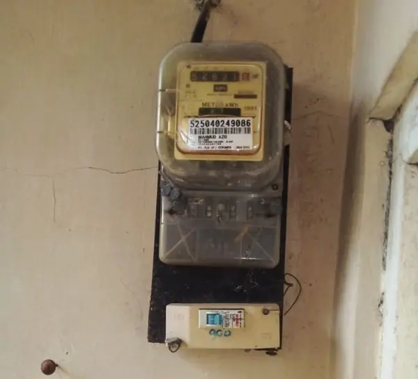
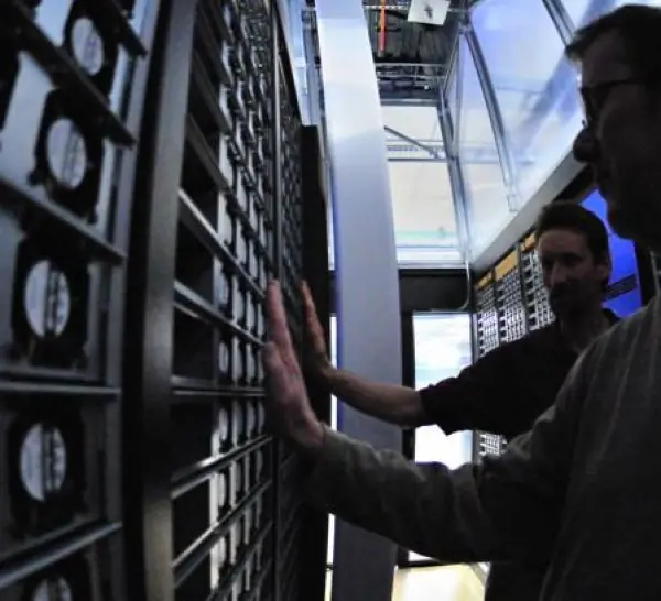
Cloud pricing copies the older utility bill. Plate 7.1 shows the three things behind a monthly invoice: a meter that measures use, a cash register that records the sale, and the racked servers that actually burn the electricity.

(a) Meter: measured service

(b) Register: record of every sale

(c) Servers: the cost behind the price

7.7.1 Eight FinOps practices to control cloud cost

1. Tag every resource. Add tags such as team, project and environment so each rupee of the bill has an owner. A college can then see that the admission portal costs more than the library site. Untagged spend is the first thing to hunt for.
2. Set budgets and alerts. Define a monthly budget and send an alert at 50, 80 and 100 percent. A forgotten test server or a runaway loop is caught in days, not at month end. This is the cheapest control to set up.
3. Right-size resources. Check real CPU and memory use and move to a smaller instance when it is idle most of the time. Many servers run below 20 percent load. Right-sizing often saves 20 to 40 percent with no change in service.
4. Switch off what is not used. Stop development and test servers at night and during holidays, and delete old disks and snapshots. A server that runs only 10 hours on working days costs a third of one that never stops. Automation makes this routine.
5. Commit for steady load. Buy reserved capacity or savings plans for the base load that runs all year, such as a database. The break-even is near 60 percent use in the book's example. Do not commit for load you cannot predict.
6. Use spot for flexible work. Batch jobs, rendering and test pipelines that can restart can use spare capacity at a large discount. Design them to save progress and handle interruption. This can cut compute cost by more than half.
7. Use storage tiers and lifecycle rules. Move old data from hot to infrequent and archive tiers automatically. Last year's scanned forms rarely need fast access. Lifecycle rules save money without anyone remembering to do it.
8. Review cost every month. Engineering, finance and management look at the bill together, learn why it changed and set targets such as cost per student or per transaction. Cost becomes a design question, not a surprise. This habit is the core of FinOps.

7.8 Summary and exercises

Cloud cost depends on the pricing model and utilisation; SLA nines translate to minutes of downtime; serial dependencies lower and parallel replicas raise availability; commitments pay off above a break-even utilisation; FinOps makes this a continuous practice.

1. Compute the yearly downtime for 99.95% availability.
2. Three services in series have 99.9%, 99.5% and 99.99%. Find the composite availability.
3. Two independent instances of 99.5% are run in parallel behind a 99.99% load balancer. Compute the availability.
4. Instance A costs 0.20 per hour on demand or 0.11 per hour reserved for all 8,760 hours. What is the break-even utilisation?
5. Explain why egress charges can dominate the bill of a video-streaming service.
6. Describe two FinOps actions for each of the Inform, Optimise and Operate phases.

Model answers: medium (5 marks) and long (10 marks) questions

Q1 (5 marks). Explain the main cloud pricing models and when each is suitable.

Introduction. Cloud services are billed by use, but the same capacity can be bought in several ways that trade price against commitment (Figure 7.1).

Model	How it works	Price (index)	Suitable for
On-demand	Pay per second or hour, no commitment	100	Unpredictable, short-lived, new projects
Savings plan	Commit to an hourly spend for 1 to 3 years	about 70	Steady spend across changing instances
Reserved	Commit to an instance for 1 to 3 years	60 in the example	Predictable base load such as databases
Spot	Spare capacity, can be reclaimed on short notice	30 or less	Fault-tolerant batch and test work

Example. A bank runs its core database on a reserved instance, its web tier on on-demand with autoscaling and its nightly reports on spot.

Conclusion match each workload's predictability and fault tolerance to the pricing model, and mix them.

Q2 (5 marks). Calculate the availability of a three-tier application and show how redundancy improves it.

Series rule. When a request needs every tier, A = A1 x A2 x A3. For web 99.95%, application 99.9% and database 99.95%: A = 0.9995 x 0.999 x 0.9995 = 99.8001%.

With 525,600 minutes in a year, the downtime is (1 - 0.998001) x 525,600 = 1,050.5 minutes (about 17.5 hours), worse than the weakest tier alone (Figure 7.3).

Parallel rule. When either of two independent copies can serve, A = 1 - (1 - A1)(1 - A2). A pair of 99.9% instances gives 1 - 0.001 x 0.001 = 99.9999% (about 0.5 minute a year). Duplicating every tier gives 99.99985%, about 0.79 minutes a year.

Caution. Failures must be independent: instances in one rack or behind one load balancer share a dependency and stay in series.

Conclusion redundancy across independent zones multiplies reliability, but every serial dependency lowers it.

Q3 (5 marks). On-demand costs 0.10 per hour; a one-year reservation costs 0.06 per hour for all 8,760 hours. Find the break-even and decide for a workload of 6,000 hours a year.

Reserved cost = 0.06 x 8,760 = 525.60 a year, whatever the use. On-demand cost = 0.10 x hours. Break-even hours = 525.60 / 0.10 = 5,256 hours, which is 5,256 / 8,760 = 60% of the year (Figure 7.2).

Decision. At 6,000 hours: on-demand = 0.10 x 6,000 = 600.00; reserved = 525.60; the saving is 74.40, or 74.40 / 600 = 12.4%. The workload runs 68% of the time, above the 60% threshold, so reserve.

At 4,000 hours the on-demand cost of 400.00 would be lower and reserving would lose 125.60.

Conclusion reserve only for load that will certainly exceed the break-even utilisation.

Q4 (10 marks). Explain SLI, SLO and SLA. Discuss total cost of ownership (TCO) and FinOps for a cloud migration, with an availability calculation.

Introduction. Reliability and cost are the two numbers management asks about a cloud service. Engineers express reliability as SLI, SLO and SLA, and manage cost through TCO analysis and FinOps.

SLI, SLO, SLA. A Service Level Indicator (SLI) is a measured quantity, such as the percentage of requests answered successfully within 300 ms.

A Service Level Objective (SLO) is the internal target for it, for example 99.9% over 30 days; the gap to 100% is the error budget.

A Service Level Agreement (SLA) is the contract with consequences, usually service credits, if the provider falls below a stated level; it is normally looser than the SLO.

Figure 7.4 shows that 99.9% allows 525.6 minutes (8.76 hours) of downtime a year while 99.99% allows 52.6 minutes.

Composite availability. A provider's SLA for one service does not give your end-to-end availability. Serial dependencies multiply: 99.95% x 99.9% x 99.95% = 99.8001%, or 1,050 minutes a year.

Duplicating each tier across independent zones raises it to 99.99985% (Figure 7.3).

TCO. The total cost of ownership compares like with like: for an own data centre, hardware, space, power, cooling, licences, staff and refresh; for the cloud, compute, storage, network transfer, support, migration and training.

A fair comparison counts the idle capacity of fixed hardware and the cost of peaks (Plate 7.1). Cloud saves most for variable load; stable, high-utilisation load can be cheaper on reserved capacity or on owned hardware.

FinOps. Practices include tagging, budgets and alerts, right-sizing, switching off idle resources, commitments for steady load (break-even at 60% in the worked case, 5,256 hours), spot for flexible work, storage lifecycle rules and a monthly cost review (Figure 7.2).

Concept	Question it answers
SLI	What do we measure?
SLO	What do we aim for?
SLA	What do we promise, and what happens if we fail?
TCO	What does it really cost over its life?
FinOps	Who is accountable for the bill, and is it worth it?

Conclusion. A sound migration states reliability as measurable SLOs, builds redundancy where the arithmetic demands it, compares TCO honestly and runs FinOps from day one, so the cloud delivers both reliability and value.