Unit 7 · 5 teaching hours · 30 min read
Trees
What the syllabus asks for 8
- Basic terms
- Binary search tree (BST)
- Height, level, depth and tree counting facts
- AVL balanced trees
- B-trees
- The Huffman algorithm
- Game trees and minimax
- Seeing the ideas: trees, balance and compression
A tree is a non-linear structure that models hierarchy: one root, and each node has zero or more children. File systems, HTML documents, organisation charts and compiler syntax trees are trees.
- Tree terminology and the binary tree.
- Binary search tree: search, insertion, deletion, traversals, height.
- AVL trees and the four rotations; B-trees by example.
- The Huffman algorithm and game trees (minimax), each with tested code.
7.1 Basic terms
| Term | Meaning |
|---|---|
| Root | topmost node (no parent) |
| Parent / child / sibling | direct upper / lower neighbour / same parent |
| Leaf | node with no children (external node) |
| Degree | number of children of a node; degree of a tree = maximum |
| Level | root is at level 0; child level = parent level + 1 |
| Depth of a node | edges from the root to the node (= its level) |
| Height of a node | edges on the longest path down to a leaf; leaf = 0 |
| Height of a tree | height of its root; the empty tree is −1 |
| Subtree | a node together with all its descendants |
A tree with n nodes has exactly n − 1 edges. A binary tree allows at most two children per node (left and right). A binary tree of height h has at most 2^{h+1} − 1 nodes and at most 2^{h} leaves.
A full binary tree has 0 or 2 children everywhere; a complete one fills all levels except possibly the last, which fills left to right (the shape of a heap).
7.2 Binary search tree (BST)
For every node: all keys in its left subtree are smaller, all keys in its right subtree are larger (keys distinct). So search can discard half of the remaining tree at each step.
- Search(key): start at the root; go left if key < node, right if key > node, stop when found or
NULL. - Insert(key): search for it; the
NULLyou reach is where it belongs. - Delete(key): three cases: (1) leaf: remove it; (2) one child: replace the node by that child; (3) two children: replace the node's key with its inorder successor (the smallest key of the right subtree) or inorder predecessor, then delete that node (which has at most one child).
Cost is O(h): O(\log n) for a balanced tree, but O(n) if keys arrive sorted (the tree degenerates into a list). This is the motivation for AVL trees (7.4).
Traversals
| Traversal | Order | Use |
|---|---|---|
| Preorder | root, left, right | copy a tree, prefix expression |
| Inorder | left, root, right | sorted order of a BST |
| Postorder | left, right, root | delete a tree, postfix expression |
| Level order | level by level (uses a queue) | shortest-depth search |
Insert 50, 30, 70, 20, 40, 60, 80. Inorder: 20 30 40 50 60 70 80 (sorted). Preorder: 50 30 20 40 70 60 80. Postorder: 20 40 30 60 80 70 50. Height 2, 7 nodes, 6 edges. Deleting 50 (two children) replaces it by its successor 60.
#include <stdio.h>
#include <stdlib.h>

typedef struct T { int key; struct T *l, *r; } T;

T *insert(T *t, int k) {
    if (!t) { t = malloc(sizeof *t); t->key = k; t->l = t->r = NULL; return t; }
    if (k < t->key) t->l = insert(t->l, k); else if (k > t->key) t->r = insert(t->r, k);
    return t;
}
T *min_node(T *t) { while (t->l) t = t->l; return t; }
T *delete(T *t, int k) {
    if (!t) return NULL;
    if (k < t->key) t->l = delete(t->l, k);
    else if (k > t->key) t->r = delete(t->r, k);
    else if (!t->l || !t->r) { T *c = t->l ? t->l : t->r; free(t); return c; }   /* 0 or 1 child */
    else { T *s = min_node(t->r); t->key = s->key; t->r = delete(t->r, s->key); }  /* 2 children */
    return t;
}
int height(T *t) { if (!t) return -1; int a = height(t->l), b = height(t->r); return 1 + (a > b ? a : b); }
void pre(T *t)  { if (t) { printf("%d ", t->key); pre(t->l); pre(t->r); } }
void in(T *t)   { if (t) { in(t->l); printf("%d ", t->key); in(t->r); } }
void post(T *t) { if (t) { post(t->l); post(t->r); printf("%d ", t->key); } }
void level(T *t, int d) {                          /* print nodes at depth d */
    if (!t) return;
    if (d == 0) printf("%d ", t->key); else { level(t->l, d - 1); level(t->r, d - 1); }
}

int main(void) {
    T *root = NULL; int keys[] = {50, 30, 70, 20, 40, 60, 80};
    for (int i = 0; i < 7; i++) root = insert(root, keys[i]);
    printf("inorder : "); in(root);   printf("\npreorder: "); pre(root);
    printf("\npostorder: "); post(root);
    printf("\nlevel order: "); for (int d = 0; d <= height(root); d++) level(root, d);
    printf("\nheight = %d\n", height(root));
    root = delete(root, 20); printf("delete 20 (leaf)      : "); in(root); printf("| pre: "); pre(root);
    root = delete(root, 30); printf("\ndelete 30 (one child) : "); in(root); printf("| pre: "); pre(root);
    root = delete(root, 50); printf("\ndelete 50 (two child) : "); in(root); printf("| pre: "); pre(root);
    printf("\n");
    return 0;
}
inorder : 20 30 40 50 60 70 80
preorder: 50 30 20 40 70 60 80
postorder: 20 40 30 60 80 70 50
level order: 50 30 70 20 40 60 80
height = 2
delete 20 (leaf)      : 30 40 50 60 70 80 | pre: 50 30 40 70 60 80
delete 30 (one child) : 40 50 60 70 80 | pre: 50 40 70 60 80
delete 50 (two child) : 40 60 70 80 | pre: 60 40 70 80
7.3 Height, level, depth and tree counting facts
- Nodes at level k: at most 2^{k}. A tree of height h: at most 2^{h+1} − 1 nodes. Minimum height with n nodes: ⌊log₂ n⌋.
- In any binary tree, leaves = nodes with two children + 1.
- An expression tree has operands at the leaves and operators inside; its inorder, preorder and postorder traversals give infix, prefix and postfix.
7.4 AVL balanced trees
An AVL tree (Adelson-Velsky and Landis, 1962) is a BST in which, for every node, the balance factor BF = height(left) − height(right) is −1, 0 or +1. Keeping this makes the height at most about 1.44 log₂ n, so search, insert and delete are all O(\log n).
After an insertion, walk up; at the first node whose BF becomes ±2, restore balance by a rotation:
| Case | Where the new node went (relative to the unbalanced node z) | Fix |
|---|---|---|
| LL | left child's left subtree | single right rotation at z |
| RR | right child's right subtree | single left rotation at z |
| LR | left child's right subtree | left rotation at the child, then right rotation at z |
| RL | right child's left subtree | right rotation at the child, then left rotation at z |
A rotation is a local rearrangement of three pointers that preserves the inorder sequence.
Insert 10, 20: fine. Insert 30: node 10 has BF −2 (RR case) → left rotation: root 20 with children 10 and 30. Insert 40: under 30.
Insert 50: node 30 has BF −2 (RR) → left rotation: 40 becomes the parent of 30 and 50; tree: 20(10, 40(30, 50)).
Insert 25: goes under 30 (left); node 20 now has BF −2 and its right child 40 is left-heavy (RL case) → right rotation at 40, left rotation at 20. Final tree: root 30, left 20 (children 10, 25), right 40 (child 50). Preorder 30 20 10 25 40 50, height 2.
#include <stdio.h>
#include <stdlib.h>

typedef struct A { int key, h; struct A *l, *r; } A;

int H(A *t) { return t ? t->h : 0; }                     /* height counted in nodes here */
int mx(int a, int b) { return a > b ? a : b; }
void upd(A *t) { t->h = 1 + mx(H(t->l), H(t->r)); }
int bf(A *t) { return t ? H(t->l) - H(t->r) : 0; }

A *rot_right(A *z) { A *y = z->l; z->l = y->r; y->r = z; upd(z); upd(y); return y; }
A *rot_left(A *z)  { A *y = z->r; z->r = y->l; y->l = z; upd(z); upd(y); return y; }

A *insert(A *t, int k) {
    if (!t) { t = malloc(sizeof *t); t->key = k; t->h = 1; t->l = t->r = NULL; return t; }
    if (k < t->key) t->l = insert(t->l, k); else if (k > t->key) t->r = insert(t->r, k); else return t;
    upd(t);
    int b = bf(t);
    if (b > 1 && k < t->l->key)  { printf("  LL at %d\n", t->key); return rot_right(t); }
    if (b < -1 && k > t->r->key) { printf("  RR at %d\n", t->key); return rot_left(t); }
    if (b > 1 && k > t->l->key)  { printf("  LR at %d\n", t->key); t->l = rot_left(t->l); return rot_right(t); }
    if (b < -1 && k < t->r->key) { printf("  RL at %d\n", t->key); t->r = rot_right(t->r); return rot_left(t); }
    return t;
}
void pre(A *t) { if (t) { printf("%d ", t->key); pre(t->l); pre(t->r); } }
void in(A *t)  { if (t) { in(t->l); printf("%d ", t->key); in(t->r); } }

int main(void) {
    A *root = NULL; int keys[] = {10, 20, 30, 40, 50, 25};
    for (int i = 0; i < 6; i++) { printf("insert %d\n", keys[i]); root = insert(root, keys[i]); }
    printf("preorder: "); pre(root); printf("\ninorder : "); in(root);
    printf("\nroot = %d, height = %d (edges)\n", root->key, root->h - 1);
    return 0;
}
insert 10
insert 20
insert 30
  RR at 10
insert 40
insert 50
  RR at 30
insert 25
  RL at 20
preorder: 30 20 10 25 40 50
inorder : 10 20 25 30 40 50
root = 30, height = 2 (edges)
7.5 B-trees
A B-tree of order m is a balanced multiway search tree used by databases and file systems, where a node is a disk block holding many keys.
Rules: every node has at most m children (m − 1 keys); every non-root internal node has at least ⌈m/2⌉ children; the root has at least 2 children (unless it is a leaf); keys inside a node are sorted; all leaves are on the same level.
Because m is large (hundreds), the height stays tiny: a billion keys fit in height 3 or 4, so a search costs only a few disk reads.
Insertion: insert the key into the proper leaf; if the leaf overflows (m keys), split it around the median key, which moves up into the parent; splits may cascade, and a root split makes the tree one level taller (the only way height grows).
10, 20 → [10 20]. Insert 30 → overflow [10 20 30], median 20 goes up: root [20], leaves [10] and [30]. Insert 40 → [30 40]. Insert 50 → [30 40 50] overflows, median 40 goes up: root [20 40], leaves [10] [30] [50]. Insert 60 → [50 60].
Insert 70 → [50 60 70] overflows, median 60 goes up: root would be [20 40 60], which overflows, so median 40 goes up to a new root. Final: root [40]; internal nodes [20] and [60]; leaves [10] [30] [50] [70].
Height grew from 1 to 2 only because the root split.
Deletion removes the key; a node that falls below the minimum borrows a key from a sibling through the parent or merges with a sibling. A B+ tree keeps all data in linked leaves, which makes range queries fast (used by most database indexes).
7.6 The Huffman algorithm
Huffman coding compresses data by giving frequent symbols short codes and rare symbols long ones, using a prefix code (no code is a prefix of another, so decoding is unambiguous).
Method put every symbol in a priority queue by frequency; repeatedly remove the two least frequent nodes, join them under a new node whose frequency is their sum, and insert it back; stop with one tree. Left edge = 0, right edge = 1.
This greedy algorithm gives the minimum possible average code length.
Frequencies: a 5, b 9, c 12, d 13, e 16, f 45 (total 100). Merge a+b = 14; then c+d = 25; then 14+e(16) = 30; then 25+30 = 55; finally f(45)+55 = 100. Code lengths: f = 1 bit; c, d, e = 3 bits; a, b = 4 bits.
Weighted length = 45·1 + 12·3 + 13·3 + 16·3 + 5·4 + 9·4 = 45 + 36 + 39 + 48 + 20 + 36 = 224 bits per 100 symbols (2.24 bits/symbol), against 3 bits/symbol for a fixed-length code.
The exact 0/1 patterns depend on which child is called left, but the lengths do not.
#include <stdio.h>
#include <stdlib.h>
#include <string.h>

typedef struct H { char sym; int f; struct H *l, *r; } H;

H *mk(char s, int f, H *l, H *r) { H *n = malloc(sizeof *n); n->sym = s; n->f = f; n->l = l; n->r = r; return n; }

void codes(H *t, char *buf, int d, int freq[], long *total) {
    if (!t->l && !t->r) {
        buf[d] = 0;
        printf("  %c (freq %2d): %s\n", t->sym, t->f, buf);
        *total += (long)t->f * d;
        return;
    }
    buf[d] = '0'; codes(t->l, buf, d + 1, freq, total);
    buf[d] = '1'; codes(t->r, buf, d + 1, freq, total);
}

int main(void) {
    char sy[] = "abcdef"; int fr[] = {5, 9, 12, 13, 16, 45};
    H *pool[16]; int n = 6;
    for (int i = 0; i < n; i++) pool[i] = mk(sy[i], fr[i], NULL, NULL);
    while (n > 1) {                                   /* pick the two smallest */
        int a = 0, b = 1;
        if (pool[b]->f < pool[a]->f) { a = 1; b = 0; }
        for (int i = 2; i < n; i++) {
            if (pool[i]->f < pool[a]->f) { b = a; a = i; }
            else if (pool[i]->f < pool[b]->f) b = i;
        }
        H *m = mk('*', pool[a]->f + pool[b]->f, pool[a], pool[b]);
        printf("merge %d + %d = %d\n", pool[a]->f, pool[b]->f, m->f);
        int lo = a < b ? a : b, hi = a < b ? b : a;
        pool[lo] = m; pool[hi] = pool[n - 1]; n--;
    }
    char buf[32]; long total = 0;
    codes(pool[0], buf, 0, fr, &total);
    printf("weighted length = %ld bits per 100 symbols\n", total);
    return 0;
}
merge 5 + 9 = 14
merge 12 + 13 = 25
merge 14 + 16 = 30
merge 25 + 30 = 55
merge 45 + 55 = 100
  f (freq 45): 0
  c (freq 12): 100
  d (freq 13): 101
  a (freq  5): 1100
  b (freq  9): 1101
  e (freq 16): 111
weighted length = 224 bits per 100 symbols
7.7 Game trees and minimax
A game tree represents all possible sequences of moves in a two-player game: nodes are positions, edges are moves, levels alternate between MAX (our move, wants the largest score) and MIN (the opponent, wants the smallest).
Leaves carry scores. Minimax computes the value of each node from the leaves up: MAX nodes take the maximum of their children, MIN nodes the minimum.
Alpha-beta pruning skips branches that cannot change the final decision, giving the same answer with far fewer nodes (best case, roughly the square root of the nodes).
Root MAX with three MIN children whose leaves are (3, 12, 8), (2, 4, 6), (14, 5, 2). MIN values: 3, 2, 2. MAX picks 3.
With alpha-beta: after the first branch α = 3; in the second branch the first leaf 2 ≤ α, so its remaining leaves (4, 6) are pruned; in the third, leaves 14 and 5 do not decide and the leaf 2 gives 2 ≤ α.
Seven of the nine leaves are examined (the program below confirms it).
#include <stdio.h>

int leaves[3][3] = {{3, 12, 8}, {2, 4, 6}, {14, 5, 2}};
int visited = 0;

int main(void) {
    int alpha = -1000, best = -1000;
    for (int i = 0; i < 3; i++) {
        int minv = 1000;
        for (int j = 0; j < 3; j++) {
            visited++;
            if (leaves[i][j] < minv) minv = leaves[i][j];
            if (minv <= alpha) break;                  /* prune: MAX already has better */
        }
        printf("MIN node %d value (seen so far) = %d\n", i + 1, minv);
        if (minv > best) best = minv;
        if (best > alpha) alpha = best;
    }
    printf("MAX chooses %d; leaves examined = %d of 9\n", best, visited);
    return 0;
}
MIN node 1 value (seen so far) = 3
MIN node 2 value (seen so far) = 2
MIN node 3 value (seen so far) = 2
MAX chooses 3; leaves examined = 7 of 9
7.8 Seeing the ideas: trees, balance and compression
Trees are the structure of hierarchy: a university with its faculties, campuses and departments, a folder with its sub-folders, a family with its generations.
In 1962 two Soviet mathematicians, Georgy Adelson-Velsky and Evgenii Landis, published the first self-balancing search tree, which is named AVL after them.
It solved a real problem: an ordinary binary search tree built from sorted data degenerates into a chain and loses all its speed.



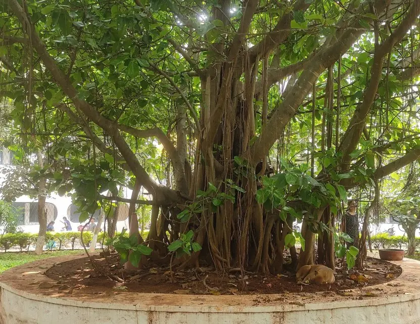
A tree is only fast when it is bushy. The banyan below is a living reminder that one trunk can spread into many branches, but a binary search tree can also grow into a single long branch if keys arrive in sorted order. The plate counts how bad that can get.

7.8.1 Eight applications of trees
- File systems. Every operating system keeps files in a tree of folders with the root at the top. A path such as
C:/College/BCA/Notesis a walk from the root to a node. Creating, deleting and searching folders are tree operations. - Organisation and hierarchy. The structure of Tribhuvan University (the university, its faculties, campuses and departments) or of Nepal's government (federal, province, local level) is a tree. An organisation chart lets a program answer questions such as "who reports to whom" quickly. Each node has exactly one parent.
- Web pages and documents. A browser turns HTML into a tree called the DOM, with the page at the root and headings, paragraphs and images below. JavaScript changes the page by editing nodes of this tree. The same idea is used for XML and JSON documents.
- Searching ordered data. A binary search tree finds a key in about log2 n comparisons when balanced: 1,000,000 records need about 20 steps. AVL and B-trees keep the tree balanced, so the speed is guaranteed. Dictionaries and sets in many languages use them.
- Database indexes. B-trees and B+ trees, which are many-way trees, keep database indexes sorted on disk. A search in a table of millions of rows, such as the voter list, needs only three or four disk reads. Banks and DBMS products use them everywhere.
- Data compression. Huffman coding builds a binary tree whose leaves are symbols and gives frequent symbols short codes (Figure 7.3). It is a part of the ZIP and JPEG formats. Saving 25 per cent of the bits, as in the example, cuts storage and download cost.
- Expression trees in compilers. A compiler stores the expression
(8 + 2) * 3as a tree with operators inside and operands at the leaves. Inorder gives the infix form, postorder gives postfix, and evaluating the tree gives the value. This links trees with the stack of Unit 2. - Game and decision trees. A game tree lists the possible moves of both players, and the minimax rule chooses the best move. Chess, tic-tac-toe and many decision systems use it. Pruning branches that cannot matter makes the search fast enough to play.
Formula and fact sheet
- n nodes → n − 1 edges. Binary tree of height h: ≤ 2^{h+1} − 1 nodes. leaves = (nodes with 2 children) + 1.
- Inorder of a BST is sorted. BST ops O(h): O(\log n) balanced, O(n) worst.
- BST delete: leaf → remove; one child → splice; two children → copy inorder successor, delete it.
- AVL: |BF| ≤ 1; rotations LL/RR single, LR/RL double; height ≤ 1.44 log₂ n.
- B-tree order m: ≤ m children, ≥ ⌈m/2⌉ children (non-root), all leaves same level.
- Huffman: greedy, merge two smallest; prefix-free, optimal.
- Minimax: MAX takes max, MIN takes min; alpha-beta prunes without changing the result.
Chapter summary
- Trees model hierarchy; binary trees limit each node to two children.
- A BST gives ordered storage and O(h) operations, and inorder traversal gives sorted output.
- AVL rotations keep the height logarithmic; B-trees keep it tiny for disk-based data.
- Huffman builds optimal prefix codes greedily; game trees with minimax and pruning choose moves.
Practice
- Define tree, binary tree, leaf, height and depth.
- Insert 45, 22, 77, 11, 30, 90, 15 into an empty BST. Give the three DFS traversals and the height.
- Delete 22 from the tree of Q2 (two children) and show the result.
- Draw the binary tree whose preorder is A B D E C F and inorder is D B E A C F.
- Insert 3, 2, 1, 4, 5, 6, 7 into an AVL tree, naming each rotation.
- Build a Huffman tree for A 40, B 30, C 15, D 10, E 5; give the code lengths and average length.
- Insert 5, 10, 15, 20, 25 into an order-3 B-tree.
- Evaluate by minimax a MAX root over two MIN nodes with leaves (4, 9) and (6, 7).
- Why can a BST be as bad as a linked list, and how does AVL prevent it?
- How many nodes can a binary tree of height 4 have at most?
Answers and worked solutions
1. Tree: hierarchical structure with one root and each node having zero or more children. Binary: ≤ 2 children. Leaf: no children. Height: edges to the deepest leaf. Depth: edges from the root.
2. BST: root 45; left 22 (children 11 → right child 15, and 30); right 77 (right child 90). Inorder: 11 15 22 30 45 77 90. Preorder: 45 22 11 15 30 77 90. Postorder: 15 11 30 22 90 77 45. Height = 3 (45 → 22 → 11 → 15).
3. Successor of 22 = smallest in right subtree = 30. Replace 22 by 30 and remove the old 30 leaf: root 45; left 30 (left subtree 11 → 15); right 77 (→ 90). Inorder: 11 15 30 45 77 90.
4. Root A (first in preorder). Inorder splits: left {D B E}, right {C F}. Left: root B, D left, E right. Right: root C, no left, F right. Tree: A(B(D, E), C(∅, F)).
5. Insert 3, 2, 1 → LL at 3 → root 2 (1, 3). Insert 4, 5 → RR at 3 → 2(1, 4(3, 5)). Insert 6 → RR at 2 → 4(2(1, 3), 5(∅, 6)). Insert 7 → RR at 5 → 4(2(1, 3), 6(5, 7)). Final balanced tree with root 4.
6. Merge E+D = 15; 15 (E+D) + C(15) = 30; 30 + B(30) = 60; 60 + A(40) = 100. Lengths: A 1, B 2, C 3, D 4, E 4. Average = (40·1 + 30·2 + 15·3 + 10·4 + 5·4)/100 = (40 + 60 + 45 + 40 + 20)/100 = 2.05 bits.
7. [5 10] → insert 15 splits: root [10], leaves [5] [15]. Insert 20 → [15 20]. Insert 25 → [15 20 25] splits: 20 up → root [10 20], leaves [5] [15] [25].
8. MIN values 4 and 6; MAX chooses 6.
9. Sorted insertions give each node only a right child, so height = n − 1 and search is O(n). AVL rotations keep |BF| ≤ 1, so height stays O(\log n).
10. 2⁵ − 1 = 31.
Model answers (5 and 10 marks)
Q1. Define a binary search tree. Construct it from the keys 50, 30, 70, 20, 40, 60, 80 and write the three traversals. (5 marks)
A binary tree is a tree in which each node has at most two children, a left child and a right child.
A binary search tree (BST) is a binary tree in which, for every node, all keys in the left subtree are smaller than the node's key and all keys in the right subtree are larger.
(Duplicates are either refused or placed consistently to one side.)
Construction (Plate 7.1b). Insert 50: it becomes the root. 30 < 50, so it goes left. 70 > 50, so it goes right. 20 < 50, < 30: left of 30. 40 < 50, > 30: right of 30. 60 > 50, < 70: left of 70. 80 > 50, > 70: right of 70.
The result is a full tree of height 2 with 7 nodes.
Traversals (Figure 7.1).
- Preorder (root, left, right): 50, 30, 20, 40, 70, 60, 80.
- Inorder (left, root, right): 20, 30, 40, 50, 60, 70, 80, which is sorted.
- Postorder (left, right, root): 20, 40, 30, 60, 80, 70, 50.
Search, insertion and deletion each take O(h) time where h is the height: O(\log n) for a balanced tree but O(n) in the worst case, when keys arrive in sorted order and the tree becomes a chain.
Q2. What is an AVL tree? Explain the rotations used to keep it balanced with an example. (5 marks)
An AVL tree is a self-balancing binary search tree in which the balance factor of every node, height(left) - height(right), is -1, 0 or +1.
If an insertion or deletion makes some node's balance factor +2 or -2, the tree is repaired by rotations, which are O(1) local changes that preserve the inorder sequence.
Because of this rule the height of an AVL tree with n nodes is at most about 1.44 log2 n, so search, insertion and deletion are all O(\log n) in the worst case.
The four cases
- Left-left (LL): the new key is inserted in the left subtree of the left child; fix with one right rotation.
- Right-right (RR): inserted in the right subtree of the right child; fix with one left rotation.
- Left-right (LR): inserted in the right subtree of the left child; fix with a left rotation on the child, then a right rotation on the node.
- Right-left (RL): inserted in the left subtree of the right child; fix with a right rotation on the child, then a left rotation on the node.
Example (Figure 7.2). Inserting 10, 20, 30 gives a chain, and node 10 has balance factor -2 (right-right case).
A left rotation at 10 makes 20 the root with children 10 and 30; every balance factor becomes 0 and the height falls from 2 to 1. The inorder order 10, 20, 30 does not change.
Q3. Explain the Huffman algorithm. Build the Huffman tree and codes for A 45, B 13, C 12, D 16, E 9, F 5 and calculate the saving. (10 marks)
Introduction. Huffman coding is a lossless compression method that gives short bit codes to frequent symbols and long codes to rare ones.
It builds a binary tree bottom-up and is an example of the greedy method, because at each step it makes the locally best choice.
The codes are prefix codes: no code is the beginning of another, so a stream of bits can be decoded without separators.
Algorithm.
- Count the frequency of each symbol and create one leaf node for each.
- Put all nodes in a priority queue (a min-heap) ordered by weight.
- While more than one node remains: remove the two nodes of smallest weight, create a new internal node whose weight is their sum with these two as children, and insert it back.
- The remaining node is the root. Label every left edge 0 and every right edge 1.
- The code of a symbol is the sequence of labels on the path from the root to its leaf.
Worked example (Figure 7.3). The merges are: F 5 + E 9 = 14; C 12 + B 13 = 25; 14 + D 16 = 30; 25 + 30 = 55; A 45 + 55 = 100. The codes are:
| Symbol | Frequency | Code | Length | Frequency x length |
|---|---|---|---|---|
| A | 45 | 0 | 1 | 45 |
| B | 13 | 101 | 3 | 39 |
| C | 12 | 100 | 3 | 36 |
| D | 16 | 111 | 3 | 48 |
| E | 9 | 1101 | 4 | 36 |
| F | 5 | 1100 | 4 | 20 |
| Total | 100 | 224 |
Saving. A fixed-length code for 6 symbols needs 3 bits each, so 100 symbols need 300 bits. Huffman needs 224 bits, an average of 2.24 bits per symbol. The saving is (300 - 224) / 300 = 25.3 per cent.
Decoding. The bit stream 0 101 1100 0 is read from the root: 0 reaches leaf A; 101 reaches B; 1100 reaches F; 0 reaches A. The decoded text is A B F A. Since no code is a prefix of another, there is only one way to read the stream.
Complexity. With a heap the algorithm takes O(n \log n) for n distinct symbols. The tree is optimal: no other prefix code has a smaller average length.
Conclusion. Huffman coding shows how a tree and a priority queue together solve a practical problem, and the same method works inside ZIP and JPEG files.