Unit 9 · 5 teaching hours · 22 min read
Searching
What the syllabus asks for 7
- Introduction to searching
- Sequential (linear) search
- Binary search
- Tree search and the general search tree
- Hashing
- Efficiency comparison
- Seeing the ideas: finding things fast
Searching is finding the record whose key equals a target, or discovering that none exists. How fast it is depends on how the data is organised: unordered, sorted, in a tree, or in a hash table.
- Sequential and binary search with exact comparison counts.
- Tree search and the general (multiway) search tree.
- Hashing: hash functions, collisions, and four collision-resolution techniques.
- A tested program and an efficiency comparison.
9.1 Introduction to searching
A search is successful if the key is found and unsuccessful otherwise. Essentials: a key to compare, a way to compare keys, and the organisation of the data. We count comparisons. Internal search works in memory; external search on files (indexes, B-trees).
9.2 Sequential (linear) search
Examine items one by one from the start. Works on any list, sorted or not. Best case 1 comparison, worst n, average about (n + 1)/2 for a successful search; O(n).
A sentinel (placing the key at the end of the array) removes the loop's bounds test. If the list is sorted, an unsuccessful search can stop early at the first larger item.
9.3 Binary search
Requires a sorted array with random access. Compare the key with the middle element; discard the half that cannot contain it; repeat. Each step halves the range, so at most ⌊log₂ n⌋ + 1 comparisons: O(\log n).
lo = 0, hi = 6: mid = 3 → 21 < 55 → lo = 4. lo = 4, hi = 6: mid = 5 → 55 found after 2 comparisons.
Searching 40: mid = 3 (21 < 40, lo = 4); mid = 5 (55 > 40, hi = 4); mid = 4 (34 < 40, lo = 5 > hi = 4) → not found after 3 comparisons. For 1,000,000 items the worst case is 20 comparisons.
9.4 Tree search and the general search tree
Searching a BST (Unit 7) is binary search on a pointer structure: O(h), i.e. O(\log n) when balanced, and unlike a sorted array it supports O(\log n) insertion and deletion.
A general (multiway) search tree generalises this: a node holds k sorted keys and k + 1 child pointers, and all keys in child i lie between key i − 1 and key i. Searching a node picks the right child by comparing against its keys.
B-trees (Unit 7) are the balanced version and are used for database indexes, since each node is one disk block. A trie is a related tree that searches strings character by character.
9.5 Hashing
Hashing computes the storage position directly from the key with a hash function h(key), giving O(1) average search, insertion and deletion. The table has m slots; the load factor α = n/m measures fullness.
Hash functions
| Method | Idea | Example (m = 100 or as stated) |
|---|---|---|
| Division | h(k) = k mod m (choose m prime, avoid powers of 2) | 1234 mod 97 = 70 |
| Mid-square | square the key, take middle digits | 123² = 15129 → 51 |
| Folding | split the key into parts and add | 123456 → 12 + 34 + 56 = 102 → 02 |
| Multiplication | h(k) = ⌊m·(k·A mod 1)⌋, A ≈ 0.618 | spreads clustered keys |
A good hash function is fast and spreads keys uniformly.
Collisions
A collision occurs when two keys hash to the same slot; it is unavoidable once keys outnumber slots (pigeonhole principle). Resolution techniques:
| Technique | How | Weakness |
|---|---|---|
| Separate chaining | each slot holds a linked list of all keys that hash there | extra memory for pointers; lists can grow |
| Linear probing (open addressing) | try h(k)+1, h(k)+2, … (mod m) | primary clustering: long runs of occupied slots |
| Quadratic probing | try h(k)+1², h(k)+2², … | secondary clustering; may not reach every slot |
| Double hashing | step size from a second hash h₂(k) | most uniform; needs h₂(k) ≠ 0 and coprime with m |
With open addressing the table can fill up, and deleting needs a tombstone marker (just emptying the slot would break the probe chain of other keys). Expected probes for linear probing: about ½(1 + 1/(1−α)) for success; chaining averages 1 + α/2.
50 → 1. 700 → 0. 76 → 6. 85 → 1 is taken → slot 2. 92 → 1, 2 taken → slot 3. 73 → 3 taken → slot 4. 101 → 3, 4 taken → slot 5. Linear probing table: [700, 50, 85, 92, 73, 101, 76]. Searching 101 follows the same probe path 3, 4, 5.
Chaining: slot 0: 700; slot 1: 50 → 85 → 92; slot 3: 73 → 101; slot 6: 76; others empty.
#include <stdio.h>
#include <stdlib.h>

#define M 7

int linear_search(const int a[], int n, int key, int *cmp) {
    for (int i = 0; i < n; i++) { (*cmp)++; if (a[i] == key) return i; }
    return -1;
}
int binary_search(const int a[], int n, int key, int *cmp) {
    int lo = 0, hi = n - 1;
    while (lo <= hi) {
        int mid = (lo + hi) / 2; (*cmp)++;
        if (a[mid] == key) return mid;
        if (a[mid] < key) lo = mid + 1; else hi = mid - 1;
    }
    return -1;
}

typedef struct Node { int key; struct Node *next; } Node;

int main(void) {
    int a[] = {3, 8, 15, 21, 34, 55, 89}, c;
    c = 0; int p = linear_search(a, 7, 55, &c); printf("linear : 55 at %d, %d comparisons\n", p, c);
    c = 0; p = binary_search(a, 7, 55, &c);     printf("binary : 55 at %d, %d comparisons\n", p, c);
    c = 0; p = binary_search(a, 7, 40, &c);     printf("binary : 40 at %d, %d comparisons\n", p, c);

    int keys[] = {50, 700, 76, 85, 92, 73, 101};
    int lp[M]; for (int i = 0; i < M; i++) lp[i] = -1;
    Node *ch[M] = {0};
    for (int i = 0; i < 7; i++) {
        int k = keys[i], h = k % M, probes = 1;
        while (lp[h] != -1) { h = (h + 1) % M; probes++; }
        lp[h] = k;
        printf("key %3d -> home %d, stored in slot %d after %d probe(s)\n", k, k % M, h, probes);
        Node *n = malloc(sizeof *n); n->key = k; n->next = NULL;      /* chaining: append to chain */
        Node **pp = &ch[k % M]; while (*pp) pp = &(*pp)->next; *pp = n;
    }
    printf("linear probing table:");
    for (int i = 0; i < M; i++) printf(" %d", lp[i]);
    printf("\nchaining:\n");
    for (int i = 0; i < M; i++) {
        printf("  slot %d:", i);
        for (Node *n = ch[i]; n; n = n->next) printf(" %d", n->key);
        printf("\n");
    }
    return 0;
}
linear : 55 at 5, 6 comparisons
binary : 55 at 5, 2 comparisons
binary : 40 at -1, 3 comparisons
key  50 -> home 1, stored in slot 1 after 1 probe(s)
key 700 -> home 0, stored in slot 0 after 1 probe(s)
key  76 -> home 6, stored in slot 6 after 1 probe(s)
key  85 -> home 1, stored in slot 2 after 2 probe(s)
key  92 -> home 1, stored in slot 3 after 3 probe(s)
key  73 -> home 3, stored in slot 4 after 2 probe(s)
key 101 -> home 3, stored in slot 5 after 3 probe(s)
linear probing table: 700 50 85 92 73 101 76
chaining:
  slot 0: 700
  slot 1: 50 85 92
  slot 2:
  slot 3: 73 101
  slot 4:
  slot 5:
  slot 6: 76
9.6 Efficiency comparison
| Method | Requirement | Search (avg / worst) | Insert | Note |
|---|---|---|---|---|
| Sequential, array | none | O(n) / O(n) | O(1) at end | simple, any order |
| Binary, sorted array | sorted | O(\log n) / O(\log n) | O(n) | needs random access |
| BST | none | O(\log n) / O(n) | O(\log n) / O(n) | ordered traversal |
| AVL / B-tree | self-balancing | O(\log n) / O(\log n) | O(\log n) | guaranteed, disk-friendly |
| Hash table | good hash, α < ~0.7 | O(1) / O(n) | O(1) | no ordering, no range queries |
9.7 Seeing the ideas: finding things fast
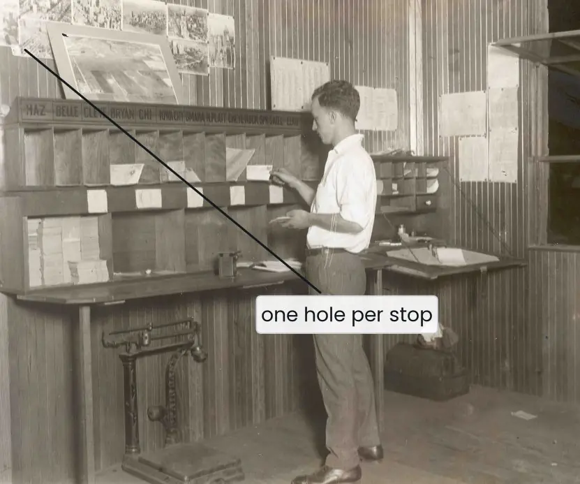
The post office sorting frame in the photograph is a hash table made of wood. The clerk does not read every letter against every address: he looks at the destination and drops the letter straight into the pigeonhole for that stop.
A hash function does exactly this for a key in memory, turning it into a table position in one step. Binary search, in contrast, uses order: it halves the search area at every comparison, like looking up a word in a dictionary.


9.7.1 Eight applications of searching and hashing
- Looking up records by key. A government portal finds a person from a citizenship number, and a bank finds an account from an account number. Hashing or an index gives the record without scanning millions of rows. Both save time for every citizen who uses the service.
- Login and password checking. A system stores a hash of each password and looks up the user by username in a hash table. The entered password is hashed and compared with the stored value. Real passwords are never kept in readable form.
- Dictionaries and spell checkers. A word processor checks every typed word against a dictionary of hundreds of thousands of words. A hash set answers "is this word present" in about one step. Binary search over a sorted word list is the alternative.
- Caches and symbol tables. A web browser keeps recently visited pages in a hash table, and a compiler keeps all variable names in one. Both need very fast insertion and lookup. Hashing gives an average of O(1) for each.
- Databases and indexes. Hash indexes support exact-match lookups, while sorted B-tree indexes support both lookup and range queries. A query such as "students with roll number 1204" uses either. The choice depends on whether ranges are needed.
- Duplicate detection. Putting each item in a hash set reveals duplicates at once, since an item that is already present is a duplicate. This is used to clean mailing lists and to remove repeated voter entries. It takes one pass over the data.
- File integrity and blockchain. A hash function such as SHA-256 maps a whole file to a short fingerprint; a changed file gives a different value. Download pages show these values so that you can check a file. Digital signatures and ledgers use the same idea.
- Searching in sorted data. Binary search finds a name in a sorted list, a page in a book or a line in a log file in O(\log n). Programmers also use it to find the first value above a limit. Its speed depends only on the data being in order.



Formula and fact sheet
- Linear search: average (n+1)/2, worst n. Binary search: ≤ ⌊log₂ n⌋ + 1.
- Load factor α = n/m. Division hash: k mod m (m prime).
- Linear probing: (h + i) mod m; quadratic: (h + i²) mod m; double: (h₁ + i·h₂) mod m.
- Chaining: expected chain length α; open addressing needs α < 1 and tombstones for deletion.
Chapter summary
- Sequential search is general but O(n); binary search is O(\log n) but needs sorted, indexable data.
- Trees add O(\log n) updates; multiway trees suit disks.
- Hashing gives O(1) average by computing the address; collisions are handled by chaining or probing.
- Choose by data order, update rate and whether ordered or range queries are needed.
Practice
- Compare sequential and binary search (requirements, cost).
- Trace binary search for 23 in [2, 5, 8, 12, 16, 23, 38, 56, 72, 91]; how many comparisons?
- Insert 12, 18, 13, 2, 3, 23, 5, 15 into a table of size 10 with h(k) = k mod 10 using linear probing.
- Do Q3 with separate chaining.
- What is a collision? Give two ways to resolve it and one drawback of each.
- Compute the folding hash of 987654 (two-digit parts, m = 100).
- Why can't we simply empty a slot when deleting in open addressing?
- For a million sorted items, how many comparisons does binary search need at most?
- Why does a hash table not support range queries efficiently?
Answers and worked solutions
1. Sequential: no ordering needed, O(n). Binary: sorted array needed, O(\log n).
2. lo 0, hi 9: mid 4 = 16 < 23 → lo 5. mid 7 = 56 > 23 → hi 6. mid 5 = 23 found: 3 comparisons.
3. 12 → 2. 18 → 8. 13 → 3. 2 → 2 taken → 3 taken → 4. 3 → 3 taken → 4 taken → 5. 23 → 3, 4, 5 taken → 6. 5 → 5 taken, 6 taken → 7. 15 → 5, 6, 7 taken → 8 taken → 9. Table: slot 2: 12, 3: 13, 4: 2, 5: 3, 6: 23, 7: 5, 8: 18, 9: 15; slots 0, 1 empty.
4. Slot 2: 12 → 2; slot 3: 13 → 3 → 23; slot 5: 5 → 15; slot 8: 18. (Order within a chain is arrival order.)
5. Two keys map to the same slot. Chaining (extra memory/pointers); linear probing (primary clustering).
6. 98 + 76 + 54 = 228 → keep two digits (mod 100) → 28.
7. An emptied slot would end the probe sequence of keys that were placed after it, making them unfindable; a tombstone marks "deleted, keep probing".
8. ⌊log₂ 1,000,000⌋ + 1 = 20.
9. Hashing scatters neighbouring keys across the table, so keys in a range are not stored together.
Model answers (5 and 10 marks)
Q1. Differentiate between linear search and binary search with algorithms. (5 marks)
Linear (sequential) search scans the items one by one from the start until the key is found or the end is reached. Binary search works on a sorted array: it compares the key with the middle item and discards the half that cannot contain it.
Linear search algorithm: for i from 0 to n - 1, if a[i] == key return i; after the loop return -1.
Binary search algorithm: set low = 0, high = n - 1. While low <= high: mid = (low + high) / 2; if a[mid] == key return mid; if a[mid] < key set low = mid + 1; otherwise set high = mid - 1. If the loop ends, return -1.
| Point | Linear search | Binary search |
|---|---|---|
| Data order | any | must be sorted |
| Time (worst) | O(n) | O(\log n) |
| Average comparisons, n = 1,000,000 | about 500,000 | at most 20 |
| Structure | array or linked list | needs direct access (array) |
| Code | very simple | slightly harder |
Example (Figure 9.1). Searching 56 in 3, 9, 14, 21, 27, 35, 42, 56, 63, 70, 81 takes four probes (mid = 5, 8, 6, 7). Linear search would need eight comparisons. Binary search is preferred for large sorted arrays; linear search is used for small or unsorted data.
Q2. What is hashing? Explain collisions and the methods of collision resolution. (5 marks)
Hashing stores and finds items by computing a table address from the key with a hash function h(key), so that on average insertion, deletion and search take O(1) time.
A common function is h(k) = k mod m for a table of m slots (m is best chosen prime). Other functions are the mid-square method and the folding method.
A collision occurs when two different keys give the same address, for example 50 mod 7 = 1 and 85 mod 7 = 1. Collisions are unavoidable, so every hash table needs a resolution method.
- Separate chaining: each slot holds a linked list of all keys that hash to it (Plate 9.1b). The table never overflows, and deletion is easy, but extra memory is used for pointers.
- Open addressing: every key lives in the table itself. When the slot is taken, another slot is probed: linear probing tries the next slot
(h + i) mod m, quadratic probing tries(h + i * i) mod m, and double hashing uses a second hash function for the step size. Linear probing is simple but causes clustering (Figure 9.2).
The load factor is the number of keys divided by the table size; chaining works well at 1 or below, while open addressing needs it kept under about 0.7, with resizing when the table fills up.
Q3. Insert the keys 50, 700, 76, 85, 92, 73, 101 into a hash table of size 7 with h(k) = k mod 7 using (a) chaining and (b) linear probing. Compare the two methods. (10 marks)
Introduction. A hash table maps keys to slots. With m = 7 the addresses are the remainders on division by 7: 50 gives 1, 700 gives 0, 76 gives 6, 85 gives 1, 92 gives 1, 73 gives 3 and 101 gives 3.
(a) Separate chaining (Plate 9.1b). Each key is added at the end of the list of its slot.
| Slot | 0 | 1 | 2 | 3 | 4 | 5 | 6 |
|---|---|---|---|---|---|---|---|
| Keys | 700 | 50, 85, 92 | empty | 73, 101 | empty | empty | 76 |
The longest chain has 3 keys. A search for 92 examines 3 nodes, a search for 76 examines 1. With n = 7 keys in m = 7 slots the load factor is 1 and a successful search needs on average 1 + 1/2 = 1.5 probes.
(b) Linear probing (Figure 9.2). On a collision try the next slot, wrapping around.
- 50 goes to slot 1 and 700 to slot 0; 76 to slot 6 (1 probe each).
- 85: slot 1 is taken, so slot 2 (2 probes).
- 92: slots 1 and 2 are taken, so slot 3 (3 probes).
- 73: slot 3 is taken, so slot 4 (2 probes).
- 101: slots 3 and 4 are taken, so slot 5 (3 probes).
The final table is 700, 50, 85, 92, 73, 101, 76 in slots 0 to 6. The total number of probes is 1 + 1 + 1 + 2 + 3 + 2 + 3 = 13. The table is full, so another key could not be inserted.
Comparison.
| Point | Chaining | Linear probing |
|---|---|---|
| Storage | keys in lists outside the table | keys inside the table |
| Table can become full | no | yes |
| Load factor allowed | above 1 | below 1 (keep under 0.7) |
| Deletion | simple | needs a special "deleted" mark |
| Clustering | none | primary clustering |
| Memory | pointer per key | none extra, but needs spare slots |
| Cache speed | slower | faster (contiguous) |
Complexity. With a good hash function and a moderate load factor, search, insertion and deletion are O(1) on average, and O(n) in the worst case when all keys collide.
Unlike a binary search tree, a hash table keeps no order among the keys, so it cannot list them sorted or answer range queries.
Conclusion. Hashing is the fastest way to find an item by exact key, as Figure 9.3 shows: about 1 probe against 20 for binary search and 500,000 for linear search on a million items.
Its quality depends on a good hash function, on keeping the load factor low, and on a sensible collision strategy.