Unit 8 · 5 teaching hours · 25 min read
Sorting
What the syllabus asks for 10
- Introduction
- Big-O notation
- The elementary sorts
- Quick sort
- Merge sort
- Heap sort
- Radix sort
- Programs: all the sorts
- Efficiency of sorting
- Seeing the ideas: sorting by machine and by method
Sorting arranges items in a defined order so that searching, merging and reporting become cheap. It is the most studied problem in computing, and it shows clearly how algorithm design decides efficiency.
- Internal versus external sorting, stability and in-place sorting.
- Insertion, selection, bubble, quick, merge, radix, shell, binary-insertion and heap sort with traces.
- Big-O, Big-Ω and Big-Θ notation, and the efficiency comparison.
- One tested program that runs all of them.
8.1 Introduction
- Internal sort: all data fits in main memory (arrays). External sort: data is on disk in blocks (too large for memory); the standard method is external merge sort: sort memory-sized chunks into runs, write them out, then merge runs with a k-way merge.
- Stable: equal keys keep their original relative order (needed when sorting by several keys in turn). In-place: uses O(1) extra memory.
- Cost is measured in comparisons and data movements.
8.2 Big-O notation
f(n) = O(g(n)) if there are constants c, n₀ with f(n) ≤ c·g(n) for all n ≥ n₀: an upper bound. Ω is a lower bound and Θ a tight bound (both). We state the worst case unless told otherwise.
f(n) = 3n² + 5n + 7. For n ≥ 1: 3n² + 5n + 7 ≤ 3n² + 5n² + 7n² = 15n², so f(n) = O(n²) with c = 15, n₀ = 1. It is also Ω(n²), hence Θ(n²). Nested loops of n iterations each give n² steps; a loop that halves n each time gives log₂ n steps.
8.3 The elementary sorts
Insertion sort. Keep a sorted prefix; take the next item and slide it left past larger items. Best case (already sorted) O(n); worst/average O(n²); stable, in place, excellent for small or nearly sorted data.
Binary insertion sort finds the slot by binary search (O(\log n) comparisons per item) but still shifts O(n) items.
Selection sort. Repeatedly select the minimum of the unsorted part and swap it to the front. Always n(n−1)/2 comparisons, but only n − 1 swaps; not stable in the usual form.
Bubble sort (exchange sort). Repeatedly compare adjacent pairs and swap if out of order; after pass k the k largest are in place. With an "already sorted" flag the best case is O(n); worst O(n²); stable.
Shell sort. Insertion sort on elements a gap apart, with the gap shrinking (n/2, n/4, …, 1). Early passes move items long distances. Runs in about O(n^{1}.3) to O(n²) depending on the gap sequence; in place, not stable.
Pass 1: (5,1) swap → 1 5 4 2 8; (5,4) swap → 1 4 5 2 8; (5,2) swap → 1 4 2 5 8; (5,8) no → largest 8 settled. Pass 2: (1,4) no; (4,2) swap → 1 2 4 5 8; (4,5) no. Pass 3: no swaps → sorted.
Insertion sort on the same data: [5] | 1 → [1 5] | 4 → [1 4 5] | 2 → [1 2 4 5] | 8 → [1 2 4 5 8].
8.4 Quick sort
Divide and conquer. Pick a pivot; partition so that smaller items are left of it and larger right; sort both sides recursively. Average O(n \log n), in place (O(\log n) stack), not stable.
Worst case O(n²) when the pivot is always the smallest or largest (e.g. first-element pivot on sorted input); random or median-of-three pivots make this rare.
i = −1. j=0: 8 > 5 skip. j=1: 3 < 5, i=0, swap a[0],a[1] → 3 8 7 1 5. j=2: 7 skip. j=3: 1 < 5, i=1, swap a[1],a[3] → 3 1 7 8 5. Finally swap pivot with a[i+1]=a[2] → 3 1 5 8 7. The pivot is in its final position; recurse on [3 1] and [8 7].
8.5 Merge sort
Split the array in halves, sort each recursively, merge the two sorted halves in linear time. T(n) = 2T(n/2) + n gives O(n \log n) in every case; stable; needs O(n) extra space. It is the basis of external sorting.
8.6 Heap sort
A max-heap is a complete binary tree stored in an array in which every parent ≥ its children (node i has children 2i+1 and 2i+2).
Build the heap bottom-up in O(n), then repeat: swap the root (the maximum) with the last element, shrink the heap, sift down the new root. O(n \log n) always, in place, not stable.
A heap is also the best implementation of a priority queue (Unit 3): insert and extract-max both O(\log n).
8.7 Radix sort
Radix sort never compares keys. It sorts digit by digit, least significant first, using a stable sort (counting or bucket) for each digit. For n numbers of d digits in base b: O(d·(n + b)), which is linear when d is constant. Stable; needs O(n + b) extra space.
Pass on units digit: 170 90 802 2 24 45 75 66. Pass on tens digit: 802 2 24 45 66 170 75 90. Pass on hundreds digit: 2 24 45 66 75 90 170 802.
8.8 Programs: all the sorts
The first program runs the four O(n²)-style sorts on one array and counts comparisons; the second runs the O(n \log n) sorts and radix sort on the same data.
#include <stdio.h>
#include <string.h>
#define N 8
static long cmp;

void show(const char *name, int *a) {
    printf("%-10s", name);
    for (int i = 0; i < N; i++) printf("%3d", a[i]);
    printf("\n");
}
void insertion(int *a) { for (int i = 1; i < N; i++) { int k = a[i], j = i - 1; while (j >= 0 && (cmp++, a[j] > k)) { a[j+1] = a[j]; j--; } a[j+1] = k; } }
void selection(int *a) { for (int i = 0; i < N-1; i++) { int m = i; for (int j = i+1; j < N; j++) { cmp++; if (a[j] < a[m]) m = j; } int t = a[i]; a[i] = a[m]; a[m] = t; } }
void bubble(int *a)    { for (int p = 0; p < N-1; p++) for (int j = 0; j < N-1-p; j++) { cmp++; if (a[j] > a[j+1]) { int t = a[j]; a[j] = a[j+1]; a[j+1] = t; } } }
void shell(int *a)     { for (int g = N/2; g > 0; g /= 2) for (int i = g; i < N; i++) { int k = a[i], j = i; while (j >= g && a[j-g] > k) { a[j] = a[j-g]; j -= g; } a[j] = k; } }

int main(void) {
    const int orig[N] = {64, 25, 12, 22, 11, 90, 5, 47};
    int a[N];
    memcpy(a, orig, sizeof a); show("original", a);
    memcpy(a, orig, sizeof a); cmp = 0; insertion(a); show("insertion", a); printf("          comparisons: %ld\n", cmp);
    memcpy(a, orig, sizeof a); cmp = 0; selection(a); show("selection", a); printf("          comparisons: %ld\n", cmp);
    memcpy(a, orig, sizeof a); cmp = 0; bubble(a);    show("bubble", a);    printf("          comparisons: %ld\n", cmp);
    memcpy(a, orig, sizeof a); shell(a);              show("shell", a);
    return 0;
}
original   64 25 12 22 11 90  5 47
insertion   5 11 12 22 25 47 64 90
          comparisons: 20
selection   5 11 12 22 25 47 64 90
          comparisons: 28
bubble      5 11 12 22 25 47 64 90
          comparisons: 28
shell       5 11 12 22 25 47 64 90
#include <stdio.h>
#include <string.h>
#define N 8
static long cmp;

void show(const char *name, int *a) {
    printf("%-10s", name);
    for (int i = 0; i < N; i++) printf("%3d", a[i]);
    printf("\n");
}

void quick(int *a, int lo, int hi) {
    if (lo >= hi) return;
    int p = a[hi], i = lo - 1;
    for (int j = lo; j < hi; j++) if (a[j] < p) { i++; int t = a[i]; a[i] = a[j]; a[j] = t; }
    int t = a[i+1]; a[i+1] = a[hi]; a[hi] = t;
    quick(a, lo, i); quick(a, i + 2, hi);
}
void merge(int *a, int lo, int mid, int hi) {
    int tmp[N], i = lo, j = mid + 1, k = lo;
    while (i <= mid && j <= hi) tmp[k++] = a[i] <= a[j] ? a[i++] : a[j++];
    while (i <= mid) tmp[k++] = a[i++];
    while (j <= hi)  tmp[k++] = a[j++];
    for (k = lo; k <= hi; k++) a[k] = tmp[k];
}
void msort(int *a, int lo, int hi) { if (lo < hi) { int m = (lo + hi) / 2; msort(a, lo, m); msort(a, m + 1, hi); merge(a, lo, m, hi); } }
void sift(int *a, int n, int i) {
    for (;;) {
        int l = 2*i + 1, r = l + 1, big = i;
        if (l < n && a[l] > a[big]) big = l;
        if (r < n && a[r] > a[big]) big = r;
        if (big == i) return;
        int t = a[i]; a[i] = a[big]; a[big] = t; i = big;
    }
}
void heapsort(int *a) {
    for (int i = N/2 - 1; i >= 0; i--) sift(a, N, i);
    for (int e = N - 1; e > 0; e--) { int t = a[0]; a[0] = a[e]; a[e] = t; sift(a, e, 0); }
}
void radix(int *a) {
    int out[N];
    for (int exp = 1; exp <= 100; exp *= 10) {
        int cnt[10] = {0};
        for (int i = 0; i < N; i++) cnt[(a[i] / exp) % 10]++;
        for (int d = 1; d < 10; d++) cnt[d] += cnt[d-1];
        for (int i = N - 1; i >= 0; i--) out[--cnt[(a[i] / exp) % 10]] = a[i];
        memcpy(a, out, sizeof out);
    }
}

int main(void) {
    const int orig[N] = {64, 25, 12, 22, 11, 90, 5, 47};
    int a[N];
    memcpy(a, orig, sizeof a); quick(a, 0, N - 1); show("quick", a);
    memcpy(a, orig, sizeof a); msort(a, 0, N - 1); show("merge", a);
    memcpy(a, orig, sizeof a); heapsort(a);        show("heap", a);
    memcpy(a, orig, sizeof a); radix(a);           show("radix", a);
    return 0;
}
quick       5 11 12 22 25 47 64 90
merge       5 11 12 22 25 47 64 90
heap        5 11 12 22 25 47 64 90
radix       5 11 12 22 25 47 64 90
8.9 Efficiency of sorting
| Algorithm | Best | Average | Worst | Extra space | Stable |
|---|---|---|---|---|---|
| Bubble (flagged) | O(n) | O(n²) | O(n²) | O(1) | yes |
| Selection | O(n²) | O(n²) | O(n²) | O(1) | no |
| Insertion | O(n) | O(n²) | O(n²) | O(1) | yes |
| Shell | O(n \log n) | ~O(n^{1}.3) | O(n²) | O(1) | no |
| Quick | O(n \log n) | O(n \log n) | O(n²) | O(\log n) | no |
| Merge | O(n \log n) | O(n \log n) | O(n \log n) | O(n) | yes |
| Heap | O(n \log n) | O(n \log n) | O(n \log n) | O(1) | no |
| Radix | O(d(n+b)) | O(d(n+b)) | O(d(n+b)) | O(n+b) | yes |
Any comparison-based sort needs at least log₂(n!) ≈ n log₂ n comparisons in the worst case, so merge and heap sort are asymptotically optimal; radix beats this bound only because it does not compare keys.
In practice libraries use hybrids (e.g. quick/insertion or merge/insertion).
8.10 Seeing the ideas: sorting by machine and by method
Sorting is among the oldest uses of machines.
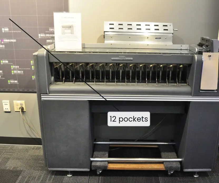
Before electronic computers, the punched cards of the 1890 census and of later business data were sorted mechanically: the IBM 082 sorter, one of the machines in the photograph, drops each card into one of twelve pockets according to a digit in one chosen column, and the operator repeats the pass for the next column.
This is exactly the radix sort of Section 8.7, performed with steel and paper. The method of quick sort, which is the fastest general method in practice, was invented in 1959 by Tony Hoare while he was a young programmer in Moscow.



8.10.1 Eight applications of sorting
- Searching faster. Binary search needs a sorted array and finds a key among 1,000,000 items in 20 steps. Sorting once and searching many times is cheaper than scanning each time. Electoral rolls and student registers are kept sorted for this reason.
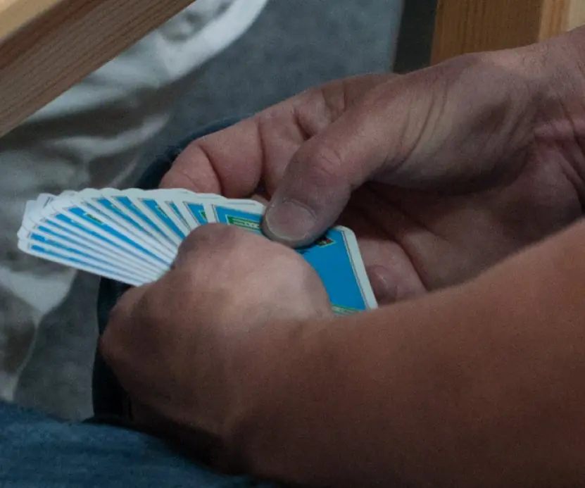
- Merit lists and rank lists. A TU or entrance-examination merit list is a list sorted by marks in descending order. Ties are broken by a second key, so the sort must be able to use several keys. A stable sort keeps equal entries in their old order.
- Databases. The
ORDER BYclause of SQL sorts the rows of a result, and sorted indexes make queries fast. Merge-based external sorting orders tables that are larger than memory. Every bank statement you view is sorted by date. - Finding duplicates and statistics. After sorting, equal items stand together, so duplicates are found in one pass. The median, the quartiles and the mode of a data set are also easy to find in a sorted list. Statisticians use this daily.
- Computer graphics. A renderer sorts objects by distance from the camera so that near objects hide far ones. Sorting makes games and maps display correctly. Without it, the picture would show things in the wrong order.
- Merging data. Two sorted lists can be merged in a single pass, which is the heart of merge sort. This is how a bank combines daily transaction files into one ledger. Sorting before merging keeps the work linear.
- Scheduling and priority work. Operating systems sort tasks by deadline or priority, and heap sort gives the next task in O(\log n). Delivery and ride-hailing services sort requests by distance or waiting time. The next job is always taken from the front.
- Library and directory order. Books on a shelf, words in a dictionary and files in a folder are sorted by title, name or date. The order lets users find an item without a search tool. This is the oldest use of sorting, long before computers.


Formula and fact sheet
- Selection: n(n−1)/2 comparisons, n−1 swaps. Bubble/insertion worst: n(n−1)/2.
- Quick: average 1.39 n log₂ n comparisons; worst n²/2. Merge: T(n) = 2T(n/2) + n.
- Heap: children of i are 2i+1, 2i+2; parent ⌊(i−1)/2⌋; build O(n).
- Comparison sorts: Ω(n \log n). Stable: bubble, insertion, merge, radix.
- Big-O: upper bound; Ω: lower; Θ: tight.
Chapter summary
- Elementary sorts are O(n²) but simple; insertion sort is the best of them for small or nearly sorted input.
- Quick, merge and heap sort reach O(n \log n); quick is fastest on average but has an O(n²) worst case, merge is stable, heap is in place.
- Radix sort is linear for fixed-width keys; external sort merges sorted runs from disk.
- Big-O describes how cost grows, not exact time.
Practice
- Differentiate internal and external sorting; what is a stable sort?
- Sort 29 10 14 37 13 by insertion sort, showing each pass.
- Trace selection sort on 64 25 12 22 11 and count comparisons and swaps.
- Perform quick sort partition on 50 30 70 20 60 with the last element as pivot.
- Show the merge steps for 38 27 43 3 9 82 10.
- Build a max-heap from 4 10 3 5 1 and give the array.
- Radix-sort 329 457 657 839 436 720 355.
- Prove 2n² + 3n = O(n²) by exhibiting c and n₀.
- Which sort would you use foranearly sorted data,bguaranteed O(n \log n) with O(1) space,ca million 6-digit integers?
- When does quick sort degrade to O(n²)?
Answers and worked solutions
1. Internal: data in memory; external: data on disk, sorted as runs then merged. Stable: equal keys keep their input order.
2. Start [29]. Insert 10 → [10 29]. Insert 14 → [10 14 29]. Insert 37 → [10 14 29 37]. Insert 13 → [10 13 14 29 37].
3. Pass 1: min 11 swapped with 64 → 11 25 12 22 64 (4 comparisons). Pass 2: min 12 ↔ 25 → 11 12 25 22 64 (3). Pass 3: min 22 ↔ 25 → 11 12 22 25 64 (2). Pass 4: 25 < 64 no swap (1). Total 10 comparisons (= 5·4/2), 3 effective swaps.
4. Pivot 60. j=0: 50 < 60, i=0 (swap with itself). j=1: 30, i=1. j=2: 70 no. j=3: 20, i=2, swap a[2],a[3] → 50 30 20 70 60. Place pivot: swap a[3] and a[4] → 50 30 20 60 70. Left [50 30 20], right [70].
5. Split: [38 27 43 3] [9 82 10] → [38 27] [43 3] [9] [82 10] → merge pairs: [27 38] [3 43] [9] [10 82] → [3 27 38 43] [9 10 82] → [3 9 10 27 38 43 82].
6. Array 4 10 3 5 1; sift down index 1 (10): children 5, 1, fine; index 0 (4): larger child 10 → swap → 10 4 3 5 1; continue at index 1: children 5, 1 → swap 4 and 5 → 10 5 3 4 1.
7. Units: 720 355 436 457 657 329 839. Tens: 720 329 436 839 355 457 657. Hundreds: 329 355 436 457 657 720 839.
8. For n ≥ 1: 3n ≤ 3n², so 2n² + 3n ≤ 5n²: c = 5, n₀ = 1.
9.(a) Insertion sort (O(n) when nearly sorted).(b) Heap sort.(c) Radix sort (6 digits, linear).
10. When the pivot is repeatedly the minimum or maximum, e.g. a first- or last-element pivot on already sorted data: partitions of sizes 0 and n − 1 give n + (n−1) + … = O(n²).
Model answers (5 and 10 marks)
Q1. Explain bubble sort with an algorithm and trace it for 5, 1, 4, 2, 8. State its complexity. (5 marks)
Bubble sort repeatedly compares adjacent items and swaps them if they are in the wrong order. After each pass the largest remaining item has "bubbled" to the end of the unsorted part.
Algorithm
- For
passfrom 1 ton - 1: setswapped = 0. - For
jfrom 0 ton - pass - 1: ifa[j] > a[j + 1], swap them and setswapped = 1. - If
swappedis 0 after a pass, stop, because the array is sorted.
Trace for 5, 1, 4, 2, 8
- Pass 1: (5,1) swap: 1 5 4 2 8; (5,4) swap: 1 4 5 2 8; (5,2) swap: 1 4 2 5 8; (5,8) no swap. Result: 1 4 2 5 8.
- Pass 2: (1,4) no; (4,2) swap: 1 2 4 5 8; (4,5) no. Result: 1 2 4 5 8.
- Pass 3: (1,2) no; (2,4) no; no swap, so the algorithm stops with 1 2 4 5 8.
Complexity. Worst and average time are O(n squared), about n(n - 1) / 2 comparisons (499,500 for n = 1,000). The best case, an already sorted array, is O(n) thanks to the swapped flag. Space is O(1) and the sort is stable and in place.
It is simple to teach but too slow for large data (Figure 8.3).
Q2. Explain quick sort with the partition step. Give its best, average and worst-case time. (5 marks)
Quick sort (Tony Hoare, 1959) is a divide-and-conquer method. It picks a pivot, partitions the array so that smaller items lie on the left of the pivot and larger items on the right, and then sorts the two parts recursively. The pivot is then in its final position.
Algorithm. quicksort(a, low, high): if low < high, set p = partition(a, low, high), then call quicksort(a, low, p - 1) and quicksort(a, p + 1, high).
Partition (Lomuto). Take a[high] as the pivot and keep an index i = low - 1. For j from low to high - 1, if a[j] <= pivot then increase i and swap a[i] with a[j]. Finally swap a[i + 1] with the pivot and return i + 1.
Example (Figure 8.2). For 10, 80, 30, 90, 40, 50, 70 with pivot 70, the items 10, 30, 40, 50 move to the small region and the final swap gives 10 30 40 50 | 70 | 90 80; 70 is at index 4 for good.
Complexity
- Best and average: O(n \log n), when the pivot splits the array roughly in half.
- Worst: O(n squared), when the pivot is always the smallest or largest item, for example a sorted array with the last item as pivot. Choosing a random or median-of-three pivot makes this very unlikely.
- Space: O(\log n) for the recursion stack on average; the sort is in place but not stable.
In practice quick sort is often the fastest method because its inner loop is short and works on neighbouring memory.
Q3. Explain merge sort with an example and compare the common sorting algorithms. (10 marks)
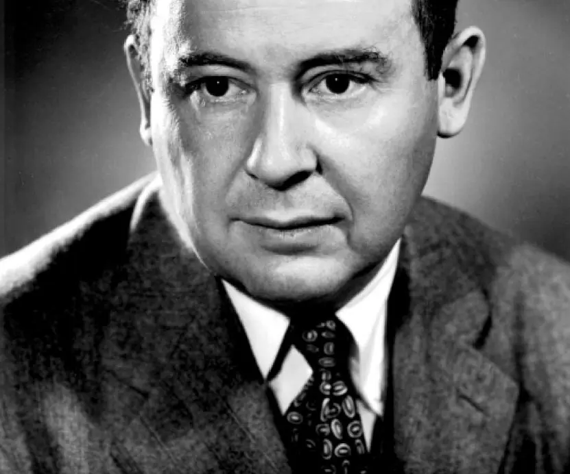
Introduction. Merge sort (John von Neumann, 1945) is a divide-and-conquer method that guarantees O(n \log n) time. Its key operation is merging two sorted lists into one sorted list in a single pass.
Algorithm. mergesort(a, low, high): (1) if low >= high, return (one item is sorted); (2) mid = (low + high) / 2; (3) mergesort(a, low, mid); (4) mergesort(a, mid + 1, high); (5) merge the two sorted halves.
Merging. Keep one pointer at the start of each half and a temporary array. Repeatedly copy the smaller of the two items under the pointers and advance that pointer; when one half is finished, copy the rest of the other.
Copy the temporary array back. Merging n items costs at most n - 1 comparisons.
Example (Figure 8.1). The array 38, 27, 43, 3, 9, 82, 10 is split into 38 27 43 3 and 9 82 10, then into 38 27, 43 3, 9 82 and 10. Merging gives 27 38, 3 43, 9 82 and 10, then 3 27 38 43 and 9 10 82, and finally 3 9 10 27 38 43 82.
Complexity. The recursion has about log2 n levels and each level does O(n) work, so the time is O(n \log n) in the best, average and worst cases. It needs O(n) extra space and is stable. It is the base of external sorting for files larger than memory.
| Algorithm | Best | Average | Worst | Space | Stable | Note |
|---|---|---|---|---|---|---|
| Bubble | O(n) | O(n squared) | O(n squared) | O(1) | yes | simple, slow |
| Selection | O(n squared) | O(n squared) | O(n squared) | O(1) | no | fewest swaps |
| Insertion | O(n) | O(n squared) | O(n squared) | O(1) | yes | good for nearly sorted |
| Quick | O(n \log n) | O(n \log n) | O(n squared) | O(\log n) | no | fastest in practice |
| Merge | O(n \log n) | O(n \log n) | O(n \log n) | O(n) | yes | guaranteed speed |
| Heap | O(n \log n) | O(n \log n) | O(n \log n) | O(1) | no | in place, guaranteed |
| Radix | O(d(n + k)) | O(d(n + k)) | O(d(n + k)) | O(n + k) | yes | integers, keys |
Conclusion. For small or nearly sorted data insertion sort is enough; for general data quick sort is usually fastest; when worst-case speed or stability is required merge sort is chosen.
For 1,000,000 items the gap between O(n squared) and O(n \log n) is the gap between 13.9 hours and 2 seconds, so the choice of algorithm matters more than the speed of the machine.