Differential Equations

A differential equation (DE) relates a function to its derivatives. Populations, cooling, circuits, vibrations and algorithms' running times all obey differential equations.

This unit covers the methods that solve the common first-order types and second-order linear equations with constant coefficients, and shows how to model with them.

6.1 Basic terms

The order of a DE is the order of the highest derivative; the degree is the power of that derivative once the equation is a polynomial in derivatives. \frac{d y}{d x} = x y is order 1, degree 1 ;\ (y'')^{2} + y' = 0 is order 2, degree 2.

The general solution has as many arbitrary constants as the order. A particular solution fixes them with initial conditions, giving an initial-value problem (IVP).

Forming a DE from a family of curves: differentiate to eliminate the constants. For y = A e^{2 x} + B e^{- x}: y' = 2 A e^{2 x} - B e^{- x} ,\ y'' = 4 A e^{2 x} + B e^{- x}.

Then y'' - y' - 2 y = 0 (check: coefficient of A: 4 - 2 - 2 = 0, of B: 1 + 1 - 2 = 0 ✓).

6.2 Separable equations

If \frac{d y}{d x} = f (x) g (y), separate: \frac{d y}{g (y)} = f (x) d x and integrate both sides.

6.3 Homogeneous equations

\frac{d y}{d x} = F \left( \frac{y}{x} \right), or more generally M and N homogeneous of the same degree. Substitute y = v x, \frac{d y}{d x} = v + \frac{x d v}{d x}; it becomes separable in v and x.

6.4 Linear first-order equations

Standard form \frac{d y}{d x} + P (x) y = Q (x). Multiply by the integrating factor \mu = e^{\int P \,d x}; the left side becomes (\mu y)', so \mu y = \int \mu Q \,d x + C.

6.5 Exact equations

M (x ,\ y) d x + N (x ,\ y) d y = 0 is exact if \frac{\partial M}{\partial y} = \frac{\partial N}{\partial x}. Then there is F with F_{x} = M ,\ F_{y} = N and the solution is F (x ,\ y) = C.

Find F by integrating M with respect to x (treating y as constant), adding a function g (y), and matching F_{y} = N.

6.6 Second-order linear equations with constant coefficients

a y'' + b y' + c y = 0. Try y = e^{m x}: it gives the auxiliary (characteristic) equation a m^{2} + b m + c = 0. The roots decide the solution:

Roots	General solution
Real, distinct m_{1} \neq m_{2}	y = C_{1} e^{m_{1} x} + C_{2} e^{m_{2} x}
Real, repeated m	y = (C_{1} + C_{2} x) e^{m x}
Complex \alpha \pm i \beta	y = e^{\alpha x} (C_{1} \cos \beta x + C_{2} \sin \beta x)

Non-homogeneous equation a y'' + b y' + c y = f (x): the general solution is y = y_{c} + y_{p}, where y_{c} is the solution of the homogeneous equation and y_{p} is any particular solution (found by trial form).

For y'' - 3 y' + 2 y = 4: t r y y_{p} = k, so 2 k = 4 ,\ k = 2 and y = C_{1} e^{x} + C_{2} e^{2 x} + 2.

(a) Hot drink: Newton's cooling law

(b) E. coli colonies on agar: growth

(c) Coil spring: oscillation

6.7 Modelling with differential equations

Growth and decay: \dfrac{dN}{dt} = kN \Rightarrow N = N_{0} e^{kt}. (k > 0 growth, k < 0 decay.)

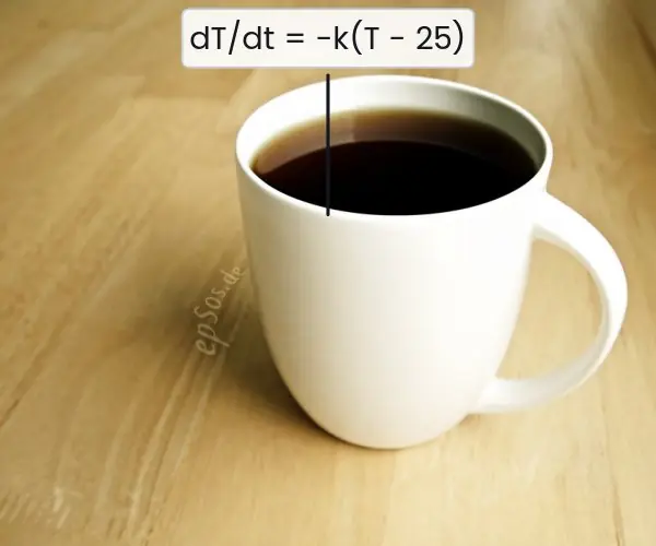
Newton's law of cooling: \dfrac{dT}{dt} = - k (T - T_{s}) \Rightarrow T (t) = T_{s} + (T_{0} - T_{s}) e^{- k t}.

Algorithms and recurrence. The divide-and-conquer recurrence T (n) = 2 T \left( \frac{n}{2} \right) + n has the continuous analogue whose solution is T (n) = n \log_{2} n; the same exponential patterns (e^{k t}) appear in compound interest, cache decay and network traffic models.

6.8 Eight uses of differential equations

1. Cooling and heating. Newton's law \dfrac{dT}{dt} = - k (T - T_{s}) tells how fast tea, a motor or a server cools (Figure 6.4a). A hostel kitchen can use it to know when soup is safe to serve. Forensic doctors use the same law to estimate the time of death.
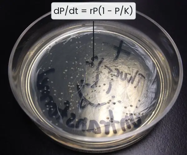
2. Population and bacteria growth. Simple growth \dfrac{dP}{dt} = kP gives exponential growth, and the logistic equation adds a limit (Figure 6.4b). Health workers use these models to predict how fast an infection spreads in a ward. City planners use them for the population of Kathmandu Valley.
3. Money and finance. Interest compounded continuously satisfies \dfrac{dA}{dt} = rA, so A = A_{0} e^{rt}. A bank in Nepal can compare a deposit that earns 8% yearly with one that compounds daily. Loan repayments with continuous payments are also modelled by a linear first-order equation.
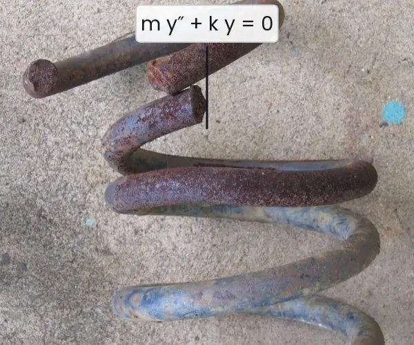
4. Spring and vibration systems. A mass on a spring obeys m y'' + c y' + k y = 0, and the roots of its characteristic equation decide the motion (Figure 6.3). Vehicle shock absorbers on rough Nepali roads are designed as critically damped systems. Earthquake engineers study the same equation for buildings.
5. Electric circuits. An RC circuit obeys \frac{R d q}{d t} + \frac{q}{C} = V and an RLC circuit is a second-order equation like the spring. The charging curve of a capacitor in a phone charger has the same shape as a cooling curve. Circuit designers use these to select resistor and capacitor values.
6. Mixing and pollution problems. If polluted water flows into a lake and clean water flows out, the amount of pollutant satisfies a linear first-order equation. Environmental officers estimate how long the Phewa lake takes to recover. A tank of salt solution in the laboratory is the classic exercise.
7. Motion with resistance. A parachutist or a vehicle with air drag obeys \frac{m d v}{d t} = mg − k v, which is separable. The speed rises towards a terminal value mg/k. This is why a hanging-glider pilot reaches a steady speed.
8. Computer simulation and games. Weather forecasts, flight simulators and physics engines in games solve differential equations step by step on a computer (Euler's and Runge-Kutta methods). Each step uses the slope field idea of Figure 6.1. The results are the animations we see on a weather map.

Formula and fact sheet

• Separable: \frac{\int d y}{g} = \int f \,d x. Homogeneous: y = v x.
• Linear: \mu = e^{\int P} ;\ \mu y = \int \mu Q + C.
• Exact: M_{y} = N_{x} ;\ F = C.
• a m^{2} + b m + c = 0: distinct → e^{m1x} ,\ e^{m2x}; repeated → (C_{1} + C_{2} x) e^{mx}; complex → eᵅˣ(cos, sin).
• Growth: N = N_{0} e^{k t}. Half-life t \frac{1}{2} = \frac{\ln 2}{k}. Cooling: T = T_{s} + (T_{0} - T_{s}) e^{- k t}.

Chapter summary

• The order sets the number of constants; initial conditions pick a particular solution.
• Separable, homogeneous, linear and exact first-order equations each have a systematic method.
• Constant-coefficient second-order equations reduce to an auxiliary quadratic whose roots give exponentials, polynomial-times-exponential, or oscillations.
• Growth, decay and cooling are first-order linear models with exponential solutions.

Practice

1. Solve \frac{d y}{d x} = \frac{y}{x} ,\ y (1) = 3.
2. Solve \frac{d y}{d x} = (1 + y^{2}) x.
3. Solve the homogeneous equation \frac{d y}{d x} = \frac{(x^{2} + y^{2})}{x y}.
4. Solve \frac{d y}{d x} + \frac{y}{x} = x^{3} and find the solution with y (1) = 1.
5. Check exactness and solve (3 x^{2} y + 2) d x + (x^{3} + 4 y) d y = 0.
6. Solve y'' + y' - 6 y = 0 ,\ y'' - 6 y' + 9 y = 0 and y'' + 9 y = 0.
7. Solve y'' - 4 y = 0 ,\ y (0) = 2 ,\ y' (0) = 0.
8. A culture of 1000 bacteria grows to 3000 in 4 hours. How many after 10 hours?
9. A body at 100 ^{\circ} C is placed in 20 ^{\circ} C surroundings and cools to 60 ^{\circ} C in 10 minutes. When does it reach 30 ^{\circ} C?
10. Form the differential equation of the family y = A \cos x + B \sin x.

Answers and worked solutions

1. \frac{d y}{y} = \frac{d x}{x} \Rightarrow y = Cx; y (1) = 3 ⇒ y = 3 x.

2. \frac{d y}{(1 + y^{2})} = x d x \Rightarrow \tan^{-1} y = \frac{x^{2}}{2} + c ⇒ y = \tan \left( \frac{x^{2}}{2} + c \right).

3. Put y = v x: v + x v' = \frac{(1 + v^{2})}{v} \Rightarrow x v' = \frac{1}{v} \Rightarrow v d v = \frac{d x}{x} \Rightarrow \frac{v^{2}}{2} = ln|x| + c ⇒ y^{2} = 2 x^{2} (\ln |x| + C).

Check by differentiating 2 y y' = 4 x ln|x| + 2 x + 2Cx, which equals 2 y \cdot \frac{(x^{2} + y^{2})}{x y} = \frac{2 (x^{2} + y^{2})}{x} once y^{2} is substituted ✓.

4. \mu = x ;\ (x y)' = x^{4} \Rightarrow x y = \frac{x^{5}}{5} + C \Rightarrow y = \frac{x^{4}}{5} + \frac{C}{x}. y (1) = 1: \frac{1}{5} + C = 1 \Rightarrow C = \frac{4}{5}: y = \frac{x^{4}}{5} + \frac{4}{5 x}.

5. M_{y} = 3 x^{2} = N_{x} ✓. F = x^{3} y + 2 x + g (y) ;\ F_{y} = x^{3} + g' = x^{3} + 4 y \Rightarrow g = 2 y^{2}. x^{3} y + 2 x + 2 y^{2} = C.

6. m^{2} + m - 6 = (m + 3) (m - 2): y = C_{1} e^{- 3 x} + C_{2} e^{2 x}. (m - 3)^{2} = 0: y = (C_{1} + C_{2} x) e^{3 x}. m = \pm 3 i: y = C_{1} \cos 3 x + C_{2} \sin 3 x.

7. m = \pm 2: y = C_{1} e^{2 x} + C_{2} e^{- 2 x} ;\ C_{1} + C_{2} = 2 ,\ 2 C_{1} - 2 C_{2} = 0 \Rightarrow C_{1} = C_{2} = 1: y = 2 \cosh 2 x = e^{2 x} + e^{- 2 x}.

8. N = 1000 e^{k t} ,\ e^{4 k} = 3 ,\ k = \frac{\ln 3}{4}. N (10) = 1000 \cdot 3^{2.5} = 1000 \times 15.59 ≈ 15,588.

9. T = 20 + 80 e^{- k t} ;\ 60 = 20 + 80 e^{- 10 k} \Rightarrow e^{- 10 k} = \frac{1}{2} ,\ k = \frac{\ln 2}{10}. T = 30: 80 e^{- k t} = 10 \Rightarrow e^{- k t} = \frac{1}{8} \Rightarrow t = 3 \times 10 = 30 minutes.

10. y'' = - A \cos x - B \sin x = - y, so y'' + y = 0.

Model answers: medium (5 marks) and long (10 marks) questions

Q (5 marks). Solve the linear equation \frac{d y}{d x} + 2 y = x by the integrating-factor method.

A first-order linear equation has the form \frac{d y}{d x} + P (x) y = Q (x). Multiplying by a suitable factor \mu (x) turns the left side into the derivative of a product, which can then be integrated.

1. Here P = 2 and Q = x. The integrating factor is \mu = e^{\int P \,d x} = e^{2 x}.
2. Multiply the equation by e^{2 x}: e^{2 x} y' + 2 e^{2 x} y = x e^{2 x}, and the left side is exactly \frac{d}{d x} (e^{2 x} y).
3. Integrate both sides: e^{2 x} y = \int x e^{2 x} \,d x.
4. By parts (u = x ,\ d v = e^{2 x} d x) this is \frac{x e^{2 x}}{2} - \frac{e^{2 x}}{4} + C.
5. Divide by e^{2 x}: y = \frac{x}{2} - \frac{1}{4} + C e^{- 2 x}.

Check: y' = \frac{1}{2} - 2 C e^{- 2 x}, so y' + 2 y = \frac{1}{2} - 2 C e^{- 2 x} + x - \frac{1}{2} + 2 C e^{- 2 x} = x ✓. The term C e^{- 2 x} dies away, so every solution approaches the line y = \frac{x}{2} - \frac{1}{4} for large x.

Q (5 marks). A cup of tea at 80 ^{\circ} C is placed in a room at 25 ^{\circ} C and cools to 60 ^{\circ} C in 10 minutes. Use Newton's law of cooling to find when it reaches 40 ^{\circ} C.

Newton's law: the rate of cooling is proportional to the difference between the body and its surroundings, \dfrac{dT}{dt} = - k (T - 25), with k > 0 (Figure 6.4a). It is separable.

1. Separate and integrate: dT/(T − 25 ) = - k d t, so \ln (T - 25) = - k t + c, that is T = 25 + A e^{- k t}.
2. At t = 0 ,\ T = 80: A = 55, so T = 25 + 55 e^{- k t}.
3. At t = 10 ,\ T = 60: 35 = 55 e^{- 10 k}, so e^{- 10 k} = \frac{7}{11} and k = \left( \frac{1}{10} \right) \ln \left( \frac{11}{7} \right) = 0.0452 per minute.
4. For T = 40: 15 = 55 e^{- k t}, so t = \left( \frac{1}{k} \right) \ln \left( \frac{55}{15} \right) = \frac{\ln (3.667)}{0.0452} = 1.2993 / 0.0452 ≈ 28.7 minutes.

Check: at t = 30 the formula gives 25 + 55 e^{- 1.356} = 39.2 ^{\circ} C, consistent with 40 ^{\circ} C near 28.7 min. The tea never goes below 25 ^{\circ} C, the room temperature.

Q (10 marks). Define order, degree and the general and particular solutions of a differential equation. Describe the methods for solving first-order equations with one example each, and solve a second-order equation with constant coefficients including an initial-value problem.

Introduction. A differential equation (DE) is an equation involving an unknown function and its derivatives. The order is that of the highest derivative and the degree is its power.

The general solution has as many arbitrary constants as the order; a particular solution fixes them by initial conditions (Figure 6.1). Many laws of physics, biology and finance are DEs (Plate 6.1).

First-order methods (Figure 6.2).

Type	Form	Example	Solution
Separable	\frac{d y}{d x} = f (x) g (y)	\frac{d y}{d x} = x y	y = C e^{\frac{x^{2}}{2}}
Homogeneous	\frac{d y}{d x} = F \left( \frac{y}{x} \right)	\frac{d y}{d x} = \frac{x + y}{x}, put y = v x	y = x (\ln |x| + C)
Linear	y' + Py = Q	y' + 2 y = x	y = \frac{x}{2} - \frac{1}{4} + C e^{- 2 x}
Exact	M d x + N d y = 0 ,\ M_{y} = N_{x}	(2 x y + 1)dx + (x^{2} + y)dy = 0	x^{2} y + x + \frac{y^{2}}{2} = C

For the exact example M = 2 x y + 1 and N = x^{2} + y; since \frac{\partial M}{\partial y} = 2 x = \frac{\partial N}{\partial x} it is exact. Find F with F_{x} = M: F = x^{2} y + x + g (y); then F_{y} = x^{2} + g' (y) = x^{2} + y gives g = \frac{y^{2}}{2}.

Second-order equation with constant coefficients. For a y'' + b y' + c y = 0 t r y y = e^{m x}, giving the auxiliary equation a m^{2} + b m + c = 0.

The roots decide the solution: real and distinct gives C_{1} e^{m_{1} x} + C_{2} e^{m_{2} x}; repeated gives (C_{1} + C_{2} x) e^{m x}; complex \alpha \pm i \beta gives e^{\alpha x} (C_{1} \cos \beta x + C_{2} \sin \beta x) (Figure 6.3).

Example (IVP). y'' + 4 y' + 3 y = 0 ,\ y (0) = 2 ,\ y' (0) = 0. The auxiliary equation m^{2} + 4m + 3 = 0 gives m = - 1 ,\ - 3, so y = C_{1} e^{- x} + C_{2} e^{- 3 x}. From y (0) = 2: C_{1} + C_{2} = 2.

From y' (0) = 0: - C_{1} - 3 C_{2} = 0. Hence C_{2} = - 1 and C_{1} = 3, so y = 3 e^{- x} - e^{- 3 x}.

Check y (0) = 3 - 1 = 2 ✓ and y' (0) = - 3 + 3 = 0 ✓.

Modelling. Cooling, growth and spring motion lead to \dfrac{dT}{dt} = - k (T - T_{s}), \dfrac{dP}{dt} = rP(1 − P/K) and m y'' + k y = 0 respectively (Figure 6.4).

Conclusion. Identify the type first (Figure 6.2), then apply its method, then check by substituting back. This routine solves nearly every examination problem in the unit.