Sensors, Calibration, Noise and Messaging

A sensor never gives the truth; it gives a number that is related to the truth.

This unit follows one reading from the soil to the server: how the board turns a voltage into a count, how calibration turns the count into a moisture percentage, how filters remove noise, how a message is packed and delivered over a bad network, and how long the battery lasts.

Every script is run with a fixed random seed, so the numbers can be reproduced.

2.1 From soil to count: the ADC

A capacitive soil probe outputs a voltage between 0 and 3.3 V; dry soil gives a higher voltage and wet soil a lower one.

The ESP32 has a 12-bit ADC, so it divides the 3.3 V range into 2^{12} = 4096 steps and returns a count from 0 to 4095. One step is 3.3 ÷ 4095 ≈ 0.8 millivolt.

A finer converter shows smaller changes, but the sensor itself is usually the weaker link.

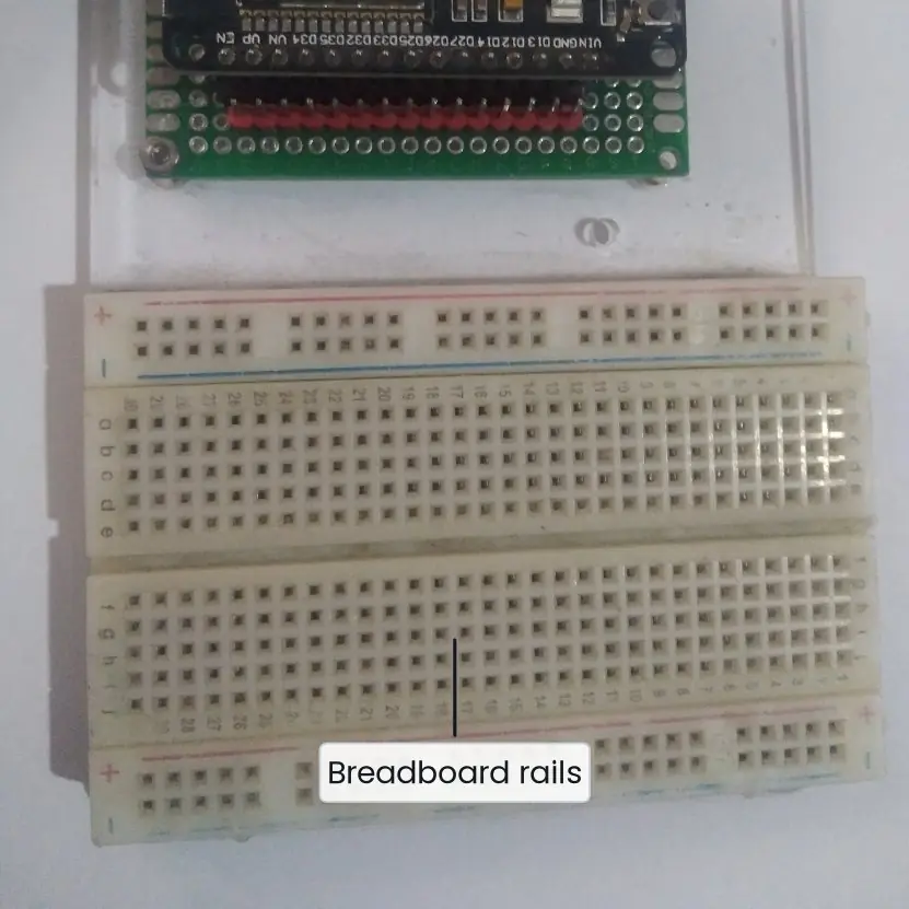
Plate 2.1 shows the wiring of a real node and its pins as a diagram.

(a) ESP32 beside a breadboard

(b) Probe wiring to the ESP32

2.2 Calibration: turning counts into moisture

The vendor's datasheet gives a rough relation, but every probe, soil and cable is different. Calibration means measuring the sensor against a trusted reference at several points and fitting a line.

The reference for soil is the oven-dry method: weigh a soil sample, dry it at 105 °C for 24 hours, weigh again, and compute the water share.

In this book the reference values and counts are simulated (the true line is count = 3100 − 38 × moisture, plus random noise with a standard deviation of 25 counts).

import numpy as np
rng = np.random.default_rng(7)
def count_for(m): return 3100 - 38 * m + rng.normal(0, 25)

ref = np.array([8, 12, 16, 20, 24, 28, 32, 36, 40, 44.0])      # oven-dry moisture, %
cnt = np.array([count_for(m) for m in ref])                      # ADC counts

a, b = np.polyfit(cnt, ref, 1)                                   # moisture = a*count + b
fit = a * cnt + b
vendor = (3100 - cnt) / (3100 - 1500) * 100                      # vendor 2-point index, 0-100
print(f"fitted line: moisture = {a:.4f} * count + {b:.2f}")
print(f"mean absolute error, fitted line : {np.mean(abs(fit - ref)):.2f} points")
print(f"mean absolute error, vendor index: {np.mean(abs(vendor - ref)):.2f} points")

test_ref = np.array([10, 18, 26, 34, 42.0])                      # 5 new samples not used in the fit
test_cnt = np.array([count_for(m) for m in test_ref])
print(f"hold-out error with fitted line  : {np.mean(abs(a * test_cnt + b - test_ref)):.2f} points")
print("O2 target (3 points) met:", np.mean(abs(a * test_cnt + b - test_ref)) <= 3)

fitted line: moisture = -0.0263 * count + 81.33
mean absolute error, fitted line : 0.32 points
mean absolute error, vendor index: 36.07 points
hold-out error with fitted line  : 0.32 points
O2 target (3 points) met: True

Reading the output. The fitted line has a mean error of 0.32 moisture points on the ten calibration samples and the same on five new samples, so objective O2 (at most 3 points) is met in simulation.

The vendor index is off by about 36 points because it is a 0 to 100 scale, not a percentage of water by volume; used without calibration it would mislead a farmer badly.

Two cautions apply to a real project: the line is only valid for one soil type (recalibrate for clay, loam and sand), and the hold-out samples must be new measurements, otherwise the error is flattered.

2.3 Noise and filters

Even a calibrated probe jitters: electrical noise, a loose wire, or a clod of soil touching the probe makes spikes. A single spike must not trigger advice.

Two simple filters are compared below on a simulated day (96 readings, true moisture falling slowly from 30 percent, noise of 1.2 points, and five spikes of +15 points).

import numpy as np
rng = np.random.default_rng(11)
t = np.arange(96)
truth = 30 - 0.05 * t
raw = truth + rng.normal(0, 1.2, 96)
for i in rng.choice(96, 5, replace=False): raw[i] += 15       # five spikes

def moving_average(x, w=5): return np.array([x[max(0, i - w + 1):i + 1].mean() for i in range(len(x))])
def moving_median(x, w=5):  return np.array([np.median(x[max(0, i - w + 1):i + 1]) for i in range(len(x))])

for name, y in (("raw", raw), ("moving average (5)", moving_average(raw)), ("moving median (5)", moving_median(raw))):
    print(f"{name:20s} mean error {np.mean(abs(y - truth)):.2f}   readings above 38 (false 'too wet'): {(y > 38).sum()}")

raw                  mean error 1.67   readings above 38 (false 'too wet'): 5
moving average (5)   mean error 1.10   readings above 38 (false 'too wet'): 0
moving median (5)    mean error 0.58   readings above 38 (false 'too wet'): 0

The moving average spreads each spike over five readings (so it lowers the spike but also drags the values around it), while the median ignores a lone spike completely.

For soil data with occasional spikes, the median is the usual first choice; it only needs an odd window and no maths.

Reading the filter output. The raw series has a mean error of 1.67 points and five false "too wet" readings.

The moving average cuts the error to 1.10 and removes the false alarms by spreading each spike over five readings; the moving median is best, with a mean error of 0.58, because a lone spike never becomes the middle value.

The price of both filters is a small delay of about two readings (30 minutes) when moisture really changes.

2.4 Messaging: publish-subscribe with retry

A node should not know who reads its data. In MQTT, a lightweight protocol, the node publishes a message to a topic such as khet/plot3/moisture, and the server subscribes to khet/+/moisture. A broker in the middle delivers.

Three quality-of-service levels trade reliability for cost.

QoS	Meaning	Cost	Use in KhetSense
0	at most once, no acknowledgement	cheapest	not suitable for the main readings
1	at least once, node retries until acknowledged	duplicates possible	chosen, with a reading id so the server drops duplicates
2	exactly once, four-step handshake	most traffic	not needed

The script below simulates 96 readings over a link that loses 30 percent of packets, in both directions. QoS 1 allows up to 3 retries and the server removes duplicates by id.

import json, random
random.seed(5)
LOSS = 0.30
def lossy(): return random.random() > LOSS            # True = packet got through

store0, store1, sent_bytes = set(), set(), 0
for i in range(96):
    msg = json.dumps({"id": i, "n": 3, "m": round(30 - 0.05 * i, 1)}, separators=(",", ":"))
    if lossy(): store0.add(i)                           # QoS 0: one try, no retry
    for attempt in range(4):                            # QoS 1: first try + 3 retries
        sent_bytes += len(msg)
        if lossy():
            store1.add(i)                               # server stores once (set removes duplicates)
            if lossy(): break                           # ack came back; stop retrying
print("payload example:", msg, f"({len(msg)} bytes)")
print(f"QoS 0 delivered {len(store0)}/96, QoS 1 delivered {len(store1)}/96, bytes sent with QoS 1: {sent_bytes}")

payload example: {"id":95,"n":3,"m":25.2} (24 bytes)
QoS 0 delivered 64/96, QoS 1 delivered 96/96, bytes sent with QoS 1: 4347

Reading the delivery output. With 30 percent loss in each direction, QoS 0 delivers only 64 of 96 readings (a third of the day is missing), while QoS 1 delivers all 96 at the cost of 4,347 bytes, about 1.9 times the traffic of one try per reading.

The payload is only 24 bytes: short keys (n for node, m for moisture) matter on a metered mobile link. Because retries can deliver a reading twice, the server must treat the id as a key and ignore repeats.

2.5 How long does the battery last?

Objective O3 asks for 30 days. Battery life is simple arithmetic: usable capacity ÷ average current. The average current is a weighted mix of the short active time and the long sleep time.

The script compares waking Wi-Fi at every reading with reading every 15 minutes but sending a batch once an hour.

CAP = 2500 * 0.8                    # 18650 cell, mAh, 80 percent usable
SLEEP = 0.15                        # mA, deep sleep incl. regulator
def avg_ma(events):                 # events: list of (mA, seconds) per 3600 s
    active = sum(i * s for i, s in events); secs = sum(s for _, s in events)
    return (active + SLEEP * (3600 - secs)) / 3600
A = [(120, 6)] * 4                                  # wake + Wi-Fi every 15 min
B = [(40, 2)] * 4 + [(120, 8)]                      # read 4 times, Wi-Fi once per hour
for name, ev in (("A: Wi-Fi every reading", A), ("B: batch each hour", B)):
    ma = avg_ma(ev)
    print(f"{name:24s} average {ma:.3f} mA  ->  {CAP / ma / 24:5.1f} days")

A: Wi-Fi every reading   average 0.949 mA  ->   87.8 days
B: batch each hour       average 0.505 mA  ->  165.1 days

Reading the battery output. Design A gives an average current of 0.949 mA and 87.8 days; design B, which sleeps between readings and uses Wi-Fi once an hour, gives 0.505 mA and 165.1 days.

Both meet objective O3 (30 days), and B leaves a wide margin for cold nights and ageing cells.

A caution: a development board with a power LED and a USB-serial chip may draw 5 to 20 mA even in "sleep", which would give only 17 to 4 days from the same cell.

Use a bare module or remove the LED and regulator losses, and always measure the real current with a multimeter.

2.6 Eight rules for reliable sensor data

1. Calibrate every probe type and soil type. A line fitted on loam is wrong for sand. Take at least 8 reference points across the working range, and keep 5 new points to test the line. State the final error in the report, as 0.32 points was stated here.
2. Read the sensor several times and take the median. One reading can be a spike from a loose wire. Take 5 readings a few milliseconds apart and send the median. This costs almost no battery because the board is already awake.
3. Let the probe settle after power-on. Many sensors give wrong values in the first 100 to 500 milliseconds. Power the probe only during the reading, wait for it to settle, then read. Powering it only when needed also reduces corrosion and current.
4. Keep messages short and structured. Use JSON with short keys, a node id, a reading id and a value. Add a version field so that the server can accept old and new nodes. A 24-byte message costs far less on a mobile data plan than a long text line.
5. Choose QoS 1 and a reading id. Retries guarantee delivery on a weak link, and the id lets the server ignore duplicates. Retry a limited number of times with a growing wait; otherwise a dead gateway drains the battery in retries.
6. Sleep as much as possible and batch the radio. The radio is the biggest user of current. Read often, send rarely, and compute the battery life for each design before buying anything, as in Section 2.5.
7. Timestamp at the server and keep the node's counter. A node without a real-time clock drifts by seconds per day. Let the server stamp the receive time and keep the node's reading id; together they allow out-of-order and late messages to be placed correctly.
8. Send a health message too. Include battery voltage and signal strength every hour. A falling voltage warns the owner days before the node dies, and a silent node (no message for 2 hours) raises an alert instead of leaving a flat line.

(a) A soil-moisture sensor pushed into the ground

(b) Raw, moving average and median filters

Formula and fact sheet

• ADC: counts = 2^bits; one step = Vref ÷ (2^bits − 1). ESP32: 12 bits, 3.3 V, about 0.8 mV per step.
• Calibration: fit moisture = a × count + b by least squares; report error on new samples.
• Median of a window ignores a lone spike; moving average smooths but is pulled by it.
• Battery life (hours) = usable mAh ÷ average mA; average mA = Σ(mA × s) ÷ 3600 over an hour.
• MQTT: topic = khet/plot3/moisture; + matches one level; QoS 0, 1, 2.

Chapter summary

• The ADC turns a voltage into a count; calibration turns the count into a useful unit and gives a measurable error.
• The simulated calibration reached 0.32 points of mean error on new samples; the uncalibrated vendor index was 36 points off.
• A moving median removed spikes best (0.58 against 1.67 for raw data).
• QoS 1 with ids delivered 96 of 96 readings on a link that lost 30 percent of packets; QoS 0 delivered 64.
• Batching the radio lengthened battery life from 87.8 to 165.1 days in the calculation.

Practice

1. How many counts does a 10-bit ADC give? What is one step on a 3.3 V range?
2. Why do capacitive soil probes give a lower voltage in wet soil?
3. Describe the oven-dry reference method in three steps.
4. Why should the hold-out samples not be used in the fit?
5. Compare a moving average and a moving median for a series with occasional spikes.
6. Write a topic name for the air temperature of the weather node and a subscription that receives all plot moisture.
7. Why must the server ignore duplicate reading ids under QoS 1?
8. A node uses 100 mA for 5 s once per hour and 0.2 mA otherwise. Find the average current.
9. With a 2,000 mAh usable cell, how many days does the node in question 8 run?
10. Why is a development board's sleep current often worse than the chip's datasheet value?

Answers and worked solutions

1. 2^{10} = 1,024 counts; one step 3.3 ÷ 1,023 ≈ 3.2 mV.

2. Water raises the permittivity of the soil, which changes the probe's oscillator so that its output voltage falls in this design.

3. Weigh a wet sample, dry it at 105 °C for 24 hours, weigh again; moisture = (wet − dry) ÷ dry × 100 (or ÷ wet, state which).

4. Testing on the training points hides over-fitting and understates the true error.

5. The average is pulled by a spike for the whole window; the median ignores one spike, so it is better for spiky data.

6. khet/weather/temp; subscription khet/+/moisture.

7. A retry after a lost acknowledgement delivers the same reading twice; counting it twice would distort averages.

8. (100 × 5 + 0.2 × 3,595) ÷ 3,600 = (500 + 719) ÷ 3,600 = 0.339 mA.

9. 2,000 ÷ 0.339 = 5,906 hours = 246 days.

10. The board adds a power LED, a USB-serial chip and a regulator that draw milliamperes even when the chip sleeps.

Model answers: medium (5 marks) and long (10 marks) questions

Q1 (5 marks). What is sensor calibration? Explain how a soil-moisture probe is calibrated and how the error is reported.

Introduction. Calibration is the process of comparing a sensor's output with a trusted reference at several known points and finding the relation that converts the raw output into a correct physical value.

Without it, a number from a datasheet can be wrong by tens of percent.

Steps.

1. Collect reference samples. Take at least 8 soil samples across the working range (for example 8 to 44 percent moisture). Insert the probe and record the ADC count, then measure the true moisture by the oven-dry method (dry at 105 °C for 24 hours and weigh).
2. Fit a line. Use least squares to find moisture = a × count + b. In the KhetSense simulation the line was moisture = −0.0263 × count + 81.33 (Figure 2.1).
3. Test on new samples. Take 5 new samples that were not used in the fit and compute the mean absolute error.
4. Report. State the error with its conditions: 0.32 points on 5 hold-out samples, for one loam soil, against the target of 3 points.

Why it matters. The uncalibrated vendor index differed from true moisture by about 36 points, so advice based on it would be wrong.

Limits The line holds for one soil type and temperature range and must be repeated for others.

Conclusion. Calibration with an independent test set is what turns a sensor reading into evidence an examiner can believe.

Q2 (5 marks). Explain publish-subscribe messaging with MQTT. Compare the QoS levels and say which suits a battery sensor node.

Introduction. In publish-subscribe messaging, a sender (publisher) does not send data directly to a receiver. It publishes to a named topic on a broker, and any client that has subscribed to the topic receives the message.

MQTT is a very light protocol of this kind, designed for small devices and weak links.

Working. A node publishes {"id":95,"n":3,"m":25.2} to khet/plot3/moisture. The server subscribes to khet/+/moisture, where + matches any single plot. New subscribers (an alert service, a dashboard) can be added without changing the node.

QoS	Guarantee	Cost
0	at most once	one packet; 64 of 96 delivered at 30 percent loss
1	at least once, duplicates possible	retries; 96 of 96 delivered, 1.9 times the bytes
2	exactly once	four-step handshake, most traffic

Choice. QoS 1 with a reading id: it survives loss, the extra traffic is small because the payload is 24 bytes, and the server removes duplicates by id. QoS 2 is unnecessary and costs battery.

Conclusion. Publish-subscribe decouples the node from the readers, and QoS 1 with idempotent storage is the practical choice for a battery-powered sensor.

Q3 (10 marks). Describe the complete data path of a sensor reading from the field to the server and explain how accuracy, noise, delivery and battery life are each handled. Use KhetSense as an example.

Introduction. A reading passes through five stages: sensing, conversion, filtering, transmission and storage. Each stage can add error or loss, so each needs a specific technique. The example is a capacitive soil probe on an ESP32 node reporting every 15 minutes.

1. Sensing and conversion. The probe outputs 0 to 3.3 V; the 12-bit ADC converts it to a count between 0 and 4095, with a step of about 0.8 mV. The probe is powered only during the reading to reduce corrosion and current.

2. Calibration. A line fitted against oven-dry samples converts counts to moisture. The simulated error was 0.32 points on new samples, satisfying objective O2 (3 points).

3. Noise handling. Five readings are taken and the median is sent; on the server a 5-point moving median removes spikes. In the test it reduced the mean error from 1.67 to 0.58 points and removed all five false "too wet" readings.

4. Transmission. A 24-byte JSON message is published to khet/plot3/moisture with QoS 1 and a reading id. On a link with 30 percent loss it delivered 96 of 96 readings against 64 for QoS 0.

5. Storage. The server stamps its own receive time, stores the reading once by id, and records gaps as missing.

6. Battery. Reading four times an hour but using Wi-Fi once, the node averages 0.505 mA and lasts 165.1 days on a 2,000 mAh usable cell, against 87.8 days when Wi-Fi is used every time.

Stage	Risk	Technique	Measured result
Conversion	wrong scale	calibration	error 0.32 points
Filtering	spikes	median	error 0.58 vs 1.67
Transmission	packet loss	QoS 1 + id	96/96 delivered
Power	short life	batching	165 days

Conclusion. Every stage of the data path has a failure and a technique to control it. A Project III report should state, for each stage, the technique used and the measured result, as the table does.