Unit 6 · Quantitative Methods · 19 teaching hours · 33 min read
Quantitative Methods in Economics (अर्थशास्त्रमा परिमाणात्मक पद्धति)
What the syllabus asks for 7
- Statistics: meaning, importance and limitations; collection of data; primary and secondary data
- Presentation of data: tables, frequency distribution and series
- Diagrammatic presentation: bar diagrams, pie chart, line graph
- Graphs of frequency distributions: histogram, frequency polygon, frequency curve and ogive
- Measures of central tendency: arithmetic mean (individual, discrete and continuous series)
- Median and quartiles
- Mode, including the empirical relation between mean, median and mode
Numbers are how economics argues. Saying that Nepali agriculture is unproductive is an opinion; saying that agriculture employs 60 per cent of the workers and produces 24 per cent of GDP is an argument. But a pile of numbers is not evidence either. It has to be collected honestly, arranged so that it can be read, presented so that it can be understood at a glance, and summarised in a few figures that stand for the whole — an average, a middle value, a most common value. Those three summaries are the measures of central tendency: the mean, the median and the mode. This unit teaches the arithmetic of all three, and the presentation of data that comes before them.
This unit is the most numerical in the paper, and the marks are the easiest in the whole subject. Group B almost always gives a series and asks for the mean, or the median, or the mode. Group C gives a continuous series and asks for the mean by the step-deviation method, or the median and the quartiles, or the mode and a check with the empirical relation Mode = 3\ Median - 2\ Mean. Learn the three tables — discrete, continuous and cumulative — and the four formulae, and the marks are yours. Always write the class interval, the mid-value and the cumulative frequency in the table; the examiner gives marks for the table.
6.1 Statistics: meaning, importance and limitations; collection of data
Statistics (तथ्याङ्कशास्त्र) has two meanings. In the plural sense, statistics are the numerical facts themselves — the figures for population, production, prices or exports. In the singular sense, statistics is the science of collecting, organising, presenting, analysing and interpreting numerical data so that decisions can be taken from it.
Importance.
- It presents facts in a definite form — a figure instead of an impression.
- It simplifies a mass of detail into a few measures such as an average or a percentage.
- It makes comparison possible between two years, two districts, two countries or two policies.
- It tests economic theories and shows whether a policy worked.
- It is the basis of policy: budgets, plans, price indices, poverty measurement and central-bank decisions are all built on statistics.
- It helps forecasting, by showing trends and by measuring the relation between one variable and another.
Limitations.
- Statistics studies groups, not individuals. It can tell you the average income of a district; it cannot tell you about one man in it.
- It deals with quantitative facts only. Honesty, beauty, loyalty and even much of welfare cannot be measured directly.
- Figures can be manipulated by an unscrupulous person, and a true figure can be made to say the opposite of the truth by leaving out the other figures. "Figures do not lie, but liars figure."
- The result is true on average only; it need not describe any single case.
- Faulty collection or a biased sample makes the whole analysis wrong: garbage in, garbage out.
- It requires trained people, and a uniform and honest method, or the figures of two offices cannot be compared.
- Statistics shows relations, not causes. A high correlation between two figures does not prove that one caused the other.
Collection of data. Data may be collected from primary or secondary sources.
| Primary data | Secondary data | |
|---|---|---|
| What it is | Data collected for the first time by the investigator himself, for his own purpose | Data already collected by somebody else and used by the investigator |
| Advantages | Original, known source, suited exactly to the purpose | Cheap, quick, and often the only source; useful for historical or national figures |
| Disadvantages | Costly, slow, needs trained staff and a good plan | May not suit the purpose; may be out of date, incomplete or inaccurate |
| Examples | A survey of household income in a village; a shop's own sales register | The population census, the national accounts, the central bank's balance of payments figures |
Methods of collecting primary data. Direct personal investigation (the investigator meets the respondent and collects the facts himself — accurate but slow and limited in area); the interview method with a schedule of questions; the questionnaire by post or e-mail (cheap and wide, but the response rate is low and the replies may be careless); the telephone interview; the panel method, in which the same respondents are studied repeatedly; and observation where the fact can be seen rather than asked about.
Method of collecting secondary data. The main sources in Nepal are the National Statistics Office (formerly the Central Bureau of Statistics) — which conducts the census and the national living standards and labour force surveys — the Nepal Rastra Bank for money, banking and balance-of-payments figures, the Ministry of Finance for the budget, the Economic Survey, departmental and municipal records, and the reports of international bodies such as the World Bank, the IMF and the UNDP. When using secondary data, always check the reliability of the source, the definitions used, the time period covered and whether the figures are complete and comparable.
6.2 Presentation of data: tables, frequency distribution and series
Data collected is raw and unreadable. The first step is to classify it — to arrange it by some characteristic, such as age, income, marks or district — and then to tabulate it, that is, to arrange it in rows and columns with a title, the units and the source.
A statistical table has five parts: the title (number, subject and period), the head note (units, if not obvious), the column headings (captions) and row headings (stubs), the body (the figures), and the footnote and source. A good table is self-explanatory: a reader should be able to understand it without reading the text.
Frequency distribution. A frequency distribution is a table that shows how many times each value or each group of values occurs.
- The variable is the characteristic being counted (marks, income, family size).
- The frequency (f) is the number of times a value occurs.
- The total frequency (N or Σf) is the number of observations.
Types of series. Data is arranged in one of three ways, and the method of finding the average depends on which it is.
1. Individual series — the values are listed one by one, without frequencies.
25, 30, 22, 35, 28, 40, 32
2. Discrete series — each value is given with its frequency; the values are whole numbers and are not grouped.
| Family size (X) | 1 | 2 | 3 | 4 | 5 |
|---|---|---|---|---|---|
| Number of families (f) | 5 | 12 | 18 | 10 | 5 |
3. Continuous series — the values are grouped into class intervals, and each interval has a frequency. The intervals must not overlap and must be of equal width where possible.
| Marks | 0–10 | 10–20 | 20–30 | 30–40 | 40–50 | 50–60 |
|---|---|---|---|---|---|---|
| Number of students (f) | 4 | 8 | 14 | 18 | 10 | 6 |
For a continuous series we use the mid-value (m) of each class, which is \frac{Lower\ limit + Upper\ limit}{2}; for the class 20–30 the mid-value is 25.
- Exclusive classes are written 0–10, 10–20, 20–30; the upper limit of one class is the lower limit of the next, and the class width is 10.
- Inclusive classes are written 1–10, 11–20, 21–30. They must be converted to exclusive classes before a graph or a median is worked out, by subtracting 0.5 from each lower limit and adding 0.5 to each upper limit.
- Open-end classes ("less than 10", "above 60") have no limit on one side; they are not used where a mean is required, because no mid-value can be found.
6.3 Diagrammatic presentation
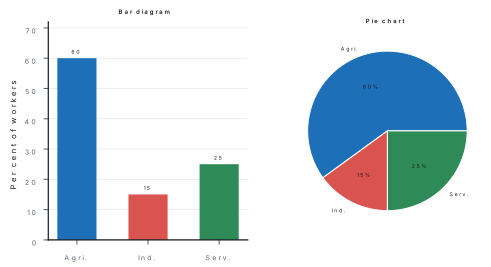
A table of figures is exact; a diagram is instant. Diagrams are used for comparison, for showing the composition of a total, and for showing a trend over time. Their uses are that they attract attention, simplify a complicated table, make comparison easy, save time, and can be understood by a person who cannot read a table. Their limitations are that they show only approximate values, they can be drawn to mislead by changing the scale, they cannot be used for any further calculation, and they need a good deal of space.
| Kind | What it shows | When to use it |
|---|---|---|
| Simple bar diagram | The value of one variable in several places or years, as vertical bars of equal width, with equal gaps | Comparing rice production in seven provinces |
| Multiple (grouped) bar diagram | Two or more variables together, as pairs or groups of bars | Comparing exports and imports for five years |
| Component (sub-divided) bar diagram | The parts of a total within one bar, usually as percentages | The share of agriculture, industry and services in GDP each year |
| Pie chart (pie diagram) | The division of a total into parts, as sectors of a circle; each sector's angle = \frac{component}{total} \times 360^\circ | The share of the budget spent on each sector in one year |
| Line graph (time series graph) | A trend over time, with time on the horizontal axis | Population growth from 1981 to 2021 |
| Pictogram | Values as repeated small pictures | Public information material |
6.4 Graphs of frequency distributions
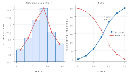
A frequency table can be turned into a picture, and the four graphs below are the standard ones. All four are drawn on the same axes: the variable on the horizontal axis and the frequency on the vertical axis.
Histogram. A histogram shows a continuous frequency distribution as a series of touching rectangles, each rectangle standing on one class interval with a height equal to that class's frequency. Because there are no gaps between classes, there are no gaps between the bars. From a histogram the mode can be read off graphically.
Frequency polygon. A frequency polygon joins the mid-points of the tops of the histogram bars by straight lines. It is drawn by taking the mid-value of each class on the horizontal axis, plotting the frequency above it, and joining the points. The two ends are closed to the mid-points of the empty classes on either side, so that the area under the polygon equals the area under the histogram.
Frequency curve. If the classes are made smaller and smaller and the number of observations is very large, the frequency polygon becomes a smooth frequency curve. Its commonest shapes are the bell-shaped (symmetrical) curve, in which the mean, median and mode all coincide; the positively skewed curve, in which the tail stretches to the right and Mode < Median < Mean; and the negatively skewed curve, in which the tail stretches to the left and Mean < Median < Mode.
Ogive (cumulative frequency curve). An ogive is drawn from cumulative frequencies. A "less than" ogive plots the upper limit of each class against the cumulative frequency up to that class, and rises from left to right; a "more than" ogive plots the lower limit against the cumulative frequency from that class upwards, and falls from left to right. Where the two curves cross, the value on the horizontal axis is the median; and reading across at N/4 and at 3N/4 gives the first and third quartiles.
6.5 Measures of central tendency: the arithmetic mean
A measure of central tendency is a single value that represents the whole series — a value around which the other values cluster. The three measures are the mean, the median and the mode. A good average should be rigidly defined, easy to understand and calculate, based on all the observations, not unduly affected by extreme values, and suitable for further algebraic treatment.
The arithmetic mean, or simply the average, is the sum of the values divided by their number. It is the most used measure because it uses every observation and can be treated algebraically, but it is badly affected by extreme values — one very large income raises the average income of a village.
Individual series.
Discrete series and continuous series.
where m is the mid-value of each class. For grouped data there are three methods:
| Method | Formula | When to use |
|---|---|---|
| Direct | \bar{X} = \frac{\Sigma f m}{\Sigma f} | Small numbers, convenient to multiply |
| Short-cut (assumed mean) | \bar{X} = A + \frac{\Sigma f d}{\Sigma f} where d = m - A | Large mid-values, to avoid big multiplications |
| Step-deviation | \bar{X} = A + \frac{\Sigma f d'}{\Sigma f} \times i where d' = \frac{m - A}{i} | Equal class intervals with large mid-values — the quickest method |
Properties worth remembering. The sum of the deviations of the values from the arithmetic mean is always zero. If every value is increased by a constant, the mean rises by that constant. The mean of a set of group means is the weighted mean, not the simple mean.
Problem. (a) Find the mean of the individual series 25, 30, 22, 35, 28, 40, 32. (b) Find the mean of the discrete series of family size. (c) Find the mean of the continuous series of marks by the step-deviation method.
| Family size (X) | 1 | 2 | 3 | 4 | 5 |
|---|---|---|---|---|---|
| Number of families (f) | 5 | 12 | 18 | 10 | 5 |
| Marks | 0–10 | 10–20 | 20–30 | 30–40 | 40–50 | 50–60 |
|---|---|---|---|---|---|---|
| Number of students (f) | 4 | 8 | 14 | 18 | 10 | 6 |
Solution. (a) Individual series. \Sigma X = 25+30+22+35+28+40+32 = 212; N = 7; \bar{X} = \frac{212}{7} = 30.29.
(b) Discrete series.
| X | f | fX |
|---|---|---|
| 1 | 5 | 5 |
| 2 | 12 | 24 |
| 3 | 18 | 54 |
| 4 | 10 | 40 |
| 5 | 5 | 25 |
| Total | 50 | 148 |
\bar{X} = \frac{\Sigma fX}{\Sigma f} = \frac{148}{50} = 2.96 persons per family.
(c) Continuous series, step-deviation method. Take the assumed mean A = 35, the mid-value of the class 30–40, and i = 10.
| Marks | f | Mid-value (m) | d' = \frac{m-35}{10} | fd' |
|---|---|---|---|---|
| 0–10 | 4 | 5 | −3 | −12 |
| 10–20 | 8 | 15 | −2 | −16 |
| 20–30 | 14 | 25 | −1 | −14 |
| 30–40 | 18 | 35 | 0 | 0 |
| 40–50 | 10 | 45 | 1 | 10 |
| 50–60 | 6 | 55 | 2 | 12 |
| Total | 60 | −20 |
\bar{X} = A + \frac{\Sigma fd'}{\Sigma f} \times i = 35 + \frac{-20}{60} \times 10 = 35 - 3.33 = 31.67 marks.
Check by the direct method: \Sigma fm = 4(5)+8(15)+14(25)+18(35)+10(45)+6(55) = 20+120+350+630+450+330 = 1{,}900; \bar{X} = \frac{1{,}900}{60} = 31.67. ✔
Answer. (a) 30.29; (b) 2.96 persons; (c) 31.67 marks. What it means. All three methods give the same answer when the arithmetic is right; the step-deviation method is simply quicker. Note that the mean of 31.67 is not one of the observed marks and need not be — an average is a value that stands for the group, not for any individual.
6.6 Median and quartiles
The median is the value of the middle item when the data is arranged in order of size. It divides the series into two equal parts: half the observations lie below it and half above.
Its advantages are that it is easy to understand, it can be found even when the classes at the ends are open-ended, and it is not affected by extreme values. Its disadvantages are that it does not use every observation, it needs the data to be arranged in order, and it is less suited to algebraic treatment.
Individual series. Arrange the values in order, then
If N is even, take the average of the \frac{N}{2}^{th} and the \left(\frac{N}{2}+1\right)^{th} items.
Discrete series. Find the cumulative frequency, then the median is the size of the \left(\frac{N+1}{2}\right)^{th} item, read against the cumulative frequency column.
Continuous series.
where L = lower limit of the median class, c.f. = cumulative frequency of the class before the median class, f = frequency of the median class, and i = the class width. The median class is the class in which \frac{N}{2} falls in the cumulative frequency column.
Quartiles. Quartiles divide the series into four equal parts. The first quartile Q_1 has a quarter of the observations below it and three quarters above; the third quartile Q_3 has three quarters below and a quarter above; Q_2 is the median itself.
The inter-quartile range = Q_3 - Q_1, and it measures the spread of the middle half of the observations.
Problem. Find the median, the first quartile and the third quartile of the marks of 60 students, and state the inter-quartile range.
| Marks | 0–10 | 10–20 | 20–30 | 30–40 | 40–50 | 50–60 |
|---|---|---|---|---|---|---|
| No. of students (f) | 4 | 8 | 14 | 18 | 10 | 6 |
Solution. Step 1 — Prepare the cumulative frequency column, and find the three required positions: \frac{N}{2} = 30, \frac{N}{4} = 15, \frac{3N}{4} = 45.
| Marks | f | c.f. |
|---|---|---|
| 0–10 | 4 | 4 |
| 10–20 | 8 | 12 |
| 20–30 | 14 | 26 |
| 30–40 | 18 | 44 |
| 40–50 | 10 | 54 |
| 50–60 | 6 | 60 |
Step 2 — Median. N/2 = 30 falls in the class 30–40 (c.f. goes from 26 to 44), so the median class is 30–40 with L = 30, c.f. = 26, f = 18, i = 10. Median = 30 + \frac{30 - 26}{18} \times 10 = 30 + 2.22 = 32.22 marks. Step 3 — First quartile. N/4 = 15 falls in the class 20–30 (c.f. goes from 12 to 26), so L = 20, c.f. = 12, f = 14, i = 10. Q_1 = 20 + \frac{15 - 12}{14} \times 10 = 20 + 2.14 = 22.14 marks. Step 4 — Third quartile. 3N/4 = 45 falls in the class 40–50 (c.f. goes from 44 to 54), so L = 40, c.f. = 44, f = 10, i = 10. Q_3 = 40 + \frac{45 - 44}{10} \times 10 = 40 + 1.00 = 41.00 marks. Step 5 — Inter-quartile range = Q_3 - Q_1 = 41.00 - 22.14 = 18.86 marks.
Answer. Median 32.22 marks; Q_1 22.14 marks; Q_3 41.00 marks; inter-quartile range 18.86 marks. What it means. Half the students scored below 32.22. The middle half of the class lies between 22.14 and 41.00 — a spread of nearly 19 marks, which tells the teacher far more about the class than the average alone: the average is 31.67, but the students are spread widely around it.
6.7 Mode and the empirical relation
The mode is the value that occurs most frequently in a series — the value that is "in fashion". For a cloth merchant the mode of shoe sizes is more useful than the average, because he must stock what sells most.
Its advantages are that it is easy to understand, it is not affected by extreme values, and it can be found even in an open-ended distribution. Its disadvantages are that it may not exist, or there may be more than one, it is not based on all the observations, and it is not suitable for further algebraic use.
Individual series. The mode is the value that appears most often.
Discrete series. The mode is the value of the variable with the highest frequency — the value whose frequency is greatest.
Continuous series. First the modal class is identified: it is the class with the highest frequency. Then
where L = lower limit of the modal class, f_1 = frequency of the modal class, f_0 = frequency of the class before it, f_2 = frequency of the class after it, and i = the class width.
The empirical relation. For a moderately asymmetrical distribution the three averages stand in a fixed order and a fixed relation:
In a symmetrical distribution all three coincide: Mean = Median = Mode. In a positively skewed distribution (the tail to the right) Mode < Median < Mean; in a negatively skewed one (the tail to the left) Mean < Median < Mode. Kiarl Pearson's coefficient of skewness measures the same thing:
Problem. Find the mode of the marks of the 60 students, and verify it with the empirical relation using the mean of 31.67 marks and the median of 32.22 marks.
| Marks | 0–10 | 10–20 | 20–30 | 30–40 | 40–50 | 50–60 |
|---|---|---|---|---|---|---|
| No. of students (f) | 4 | 8 | 14 | 18 | 10 | 6 |
Solution. Step 1 — Identify the modal class: the highest frequency is 18, in the class 30–40. So L = 30, i = 10. Step 2 — f_1 = 18 (the modal class), f_0 = 14 (the class before it), f_2 = 10 (the class after it). Step 3 — Mode = 30 + \frac{18 - 14}{2(18) - 14 - 10} \times 10. Step 4 — Mode = 30 + \frac{4}{36 - 24} \times 10 = 30 + \frac{4}{12} \times 10 = 30 + 3.33 = 33.33 marks. Step 5 — Verify with the empirical relation: Mode = 3\ Median - 2\ Mean = 3(32.22) - 2(31.67) = 96.66 - 63.34 = 33.32 marks.
Answer. Mode = 33.33 marks; the empirical relation gives 33.32, which agrees to two decimal places. What it means. The three averages are in the order Mean\ (31.67) < Median\ (32.22) < Mode\ (33.33) — that is, the distribution is negatively skewed, with a tail stretching towards the lower marks. So a few students did badly and pulled the mean down below the median and the mode, which is exactly the kind of conclusion an examiner wants from the figures.
Mean — individual \frac{\Sigma X}{N}; discrete \frac{\Sigma fX}{\Sigma f}; continuous \frac{\Sigma fm}{\Sigma f}; step-deviation A + \frac{\Sigma fd'}{\Sigma f} \times i. Median — individual \left(\frac{N+1}{2}\right)^{th} item; continuous L + \frac{\frac{N}{2}-c.f.}{f} \times i. Quartiles — same formula with \frac{N}{4} and \frac{3N}{4}. Mode — the value with the highest frequency; continuous L + \frac{f_1 - f_0}{2f_1 - f_0 - f_2} \times i. Empirical relation — Mode = 3\ Median - 2\ Mean. Skewness — symmetrical: all three equal; positive: Mode < Median < Mean; negative: Mean < Median < Mode. Pie chart — angle of a sector = \frac{component}{total} \times 360^\circ.
Five errors cost marks in this unit. First, using the upper limit of a class instead of the mid-value in the mean of a continuous series. Second, in the median formula, using the cumulative frequency including the median class instead of the class before it. Third, forgetting to convert inclusive classes (1–10, 11–20) into exclusive classes before drawing a histogram or finding the median. Fourth, mixing up the mode with the median in a discrete series: the mode is the value with the highest frequency, and the median is the value at the \left(\frac{N+1}{2}\right)^{th} position — they are often different. Fifth, in the empirical relation, writing Mode = 2\ Median - 3\ Mean or Mean = 3\ Median - 2\ Mode; the one relation to memorise is Mode = 3 Median − 2 Mean.
Chapter summary
- Statistics means either the numerical facts themselves or the science of collecting, organising, presenting, analysing and interpreting them. Its importance is in presenting facts precisely, simplifying, comparing, testing theory, guiding policy and forecasting. Its limitations are that it studies groups and not individuals, deals with quantitative facts only, can be manipulated, is true only on average, depends on the quality of collection, needs trained people, and shows relations rather than causes.
- Primary data is collected first-hand by the investigator; secondary data is already collected by somebody else. Primary methods are direct personal investigation, interview, questionnaire, telephone, panel and observation. In Nepal secondary data comes from the National Statistics Office, the Nepal Rastra Bank, the Ministry of Finance, the Economic Survey and international bodies.
- A statistical table has a title, head note, captions, stubs, body, footnote and source. A frequency distribution shows the frequency of each value or class. Series are individual, discrete or continuous; classes may be exclusive, inclusive or open-ended.
- Diagrammatic presentation — simple, multiple and component bar diagrams, the pie chart, the line graph and the pictogram — attracts attention and simplifies comparison, but shows only approximate values and can mislead.
- Graphs of frequency distributions: the histogram (touching rectangles over the classes), the frequency polygon (joining the mid-point frequencies), the frequency curve (the smooth limiting form, bell-shaped, positively or negatively skewed) and the ogive ("less than" and "more than" cumulative curves, whose crossing point gives the median).
- The arithmetic mean is \frac{\Sigma X}{N} for an individual series, \frac{\Sigma fX}{\Sigma f} for a discrete series and \frac{\Sigma fm}{\Sigma f} for a continuous series; the short-cut method uses an assumed mean and the step-deviation method uses d' = \frac{m-A}{i} and \bar{X} = A + \frac{\Sigma fd'}{\Sigma f} \times i. It uses every observation but is badly affected by extreme values.
- The median is the middle value: \left(\frac{N+1}{2}\right)^{th} item in an individual or discrete series, and Median = L + \frac{\frac{N}{2} - c.f.}{f} \times i in a continuous series. Quartiles use \frac{N}{4} and \frac{3N}{4}; the inter-quartile range is Q_3 - Q_1.
- The mode is the most frequent value: the highest frequency in a discrete series, and Mode = L + \frac{f_1 - f_0}{2f_1 - f_0 - f_2} \times i in a continuous series, where f_1 is the modal class, f_0 the class before it and f_2 the class after it.
- The empirical relation is Mode = 3\ Median - 2\ Mean. In a symmetrical distribution the three coincide; when Mode < Median < Mean the distribution is positively skewed, and when Mean < Median < Mode it is negatively skewed.
Practice questions
Group A — Very short answer (1 mark each)
- What is statistics? [1]
- Write any two importance of statistics in economics. [1]
- Distinguish between primary and secondary data in one line. [1]
- What is a frequency distribution? [1]
- What is a discrete series? [1]
- What is the mid-value of the class 20–30? [1]
- Write the formula for the arithmetic mean of an individual series. [1]
- Write the formula for the mean of a continuous series by the step-deviation method. [1]
- What is the median? [1]
- Write the formula for the median of a continuous series. [1]
- What is the mode? [1]
- State the empirical relation between mean, median and mode. [1]
- What is an ogive? [1]
- How is the angle of a sector of a pie chart found? [1]
- Which measure of central tendency is most affected by extreme values? [1]
Answers to Group A
1. Statistics is the science of collecting, organising, presenting, analysing and interpreting numerical data; in the plural sense it means the numerical facts themselves.
2. Any two of: it presents facts in a definite form; it simplifies a mass of data; it makes comparison possible; it tests theories; it guides policy; it helps forecasting.
3. Primary data is collected first-hand by the investigator for his own purpose; secondary data has already been collected by somebody else and is used by the investigator.
4. A frequency distribution is a table showing how many times each value or each class of values occurs.
5. A discrete series is one in which each value of the variable is given separately with its frequency, and the values are whole numbers not grouped into classes.
6. 25.
7. \bar{X} = \frac{\Sigma X}{N}.
8. \bar{X} = A + \frac{\Sigma fd'}{\Sigma f} \times i, where d' = \frac{m - A}{i}, m being the mid-value, A the assumed mean and i the class width.
9. The median is the value of the middle item when the data is arranged in order of size; half the observations lie below it and half above.
10. Median = L + \frac{\frac{N}{2} - c.f.}{f} \times i.
11. The mode is the value that occurs most frequently in a series.
12. Mode = 3\ Median - 2\ Mean.
13. An ogive is a graph of cumulative frequency, drawn as a "less than" or "more than" cumulative frequency curve; the point where the two curves cross gives the median.
14. Angle = \frac{component}{total} \times 360^\circ.
15. The arithmetic mean.
Group B — Short answer (5 marks each)
- What is statistics? Explain its importance and limitations in economics. [5]
- Distinguish between primary and secondary data and explain any three methods of collecting primary data. [5]
- Explain the diagrammatic presentation of data with examples. [5]
- Explain the histogram, frequency polygon and ogive. [5]
- Find the arithmetic mean of the following discrete series. [5]
| X | 5 | 10 | 15 | 20 | 25 | 30 |
|---|---|---|---|---|---|---|
| f | 4 | 6 | 10 | 12 | 5 | 3 |
- Find the mean, the median and the mode of the following continuous series. [5]
| Marks | 0–10 | 10–20 | 20–30 | 30–40 | 40–50 | 50–60 |
|---|---|---|---|---|---|---|
| f | 4 | 8 | 14 | 18 | 10 | 6 |
- Find the median and the quartiles of the series in question 6 above and state the inter-quartile range. [5]
Answers to Group B
1. Definition as in Group A answer 1. Importance: definite presentation of facts, simplification, comparison, testing of theories, guidance of policy, forecasting. Limitations: it studies groups and not individuals; it deals with quantitative facts only; figures can be manipulated; the result is true only on average; faulty collection ruins the analysis; it needs trained people and uniform methods; and it shows relations and not causes.
2. Primary data — collected first-hand by the investigator for his own purpose: original, known, exactly suited to the purpose, but costly, slow and needing trained staff. Secondary data — already collected by somebody else: cheap, quick, often the only source, but possibly unsuitable, out of date or inaccurate. Methods of collecting primary data: direct personal investigation, where the investigator meets the respondent and collects the facts himself; the interview method with a schedule; the questionnaire by post or e-mail, which is cheap and wide but has a low response rate; the telephone interview; the panel method, studying the same respondents repeatedly; and observation where the fact can be seen.
3. A diagram presents a table in a form that is understood at a glance. Kinds: simple bar diagram for comparing one variable in several places or years; multiple bar diagram for two or more variables together; component or sub-divided bar diagram for the parts of a total; pie chart, where each sector's angle is \frac{component}{total} \times 360^\circ, for showing composition; line graph for a trend over time; and pictogram. Uses: attracts attention, simplifies, makes comparison easy, saves time. Limitations: only approximate values, can mislead if the scale is manipulated, and cannot be used for further calculation.
4. Histogram — a series of touching rectangles over the class intervals, with height equal to the frequency; there are no gaps because the classes are continuous, and the mode can be read off graphically. Frequency polygon — the mid-points of the tops of the histogram bars joined by straight lines, closed at both ends to the mid-points of the neighbouring empty classes so that the area equals that of the histogram; from it the shape of the distribution is seen at once. Ogive — a cumulative frequency curve; the "less than" ogive plots the upper limit of each class against the cumulative frequency up to it and rises from left to right, and the "more than" ogive plots the lower limits against the cumulative frequency from that class upwards and falls; where the two cross, the value on the horizontal axis is the median, and reading across at N/4 and 3N/4 gives the quartiles.
5.
| X | f | fX |
|---|---|---|
| 5 | 4 | 20 |
| 10 | 6 | 60 |
| 15 | 10 | 150 |
| 20 | 12 | 240 |
| 25 | 5 | 125 |
| 30 | 3 | 90 |
| Total | 40 | 685 |
\bar{X} = \frac{685}{40} = 17.125. 6. Mean 31.67 marks (see the worked example in the text, by the direct or step-deviation method). Median 32.22 marks, using Median = 30 + \frac{30-26}{18} \times 10. Mode 33.33 marks, using Mode = 30 + \frac{18-14}{2(18)-14-10} \times 10. Check with the empirical relation: 3(32.22) - 2(31.67) = 33.32, which agrees with the mode. 7. With N = 60: N/4 = 15 falls in the class 20–30, so Q_1 = 20 + \frac{15-12}{14} \times 10 = 22.14 marks. N/2 = 30 falls in the class 30–40, so Median = 30 + \frac{30-26}{18} \times 10 = 32.22 marks. 3N/4 = 45 falls in the class 40–50, so Q_3 = 40 + \frac{45-44}{10} \times 10 = 41.00 marks. Inter-quartile range = 41.00 - 22.14 = 18.86 marks.
Group C — Long answer (8 marks each)
- What is statistics? Explain its importance and limitations, and distinguish between primary and secondary data with examples. [8]
- Find the arithmetic mean of the following continuous series by the step-deviation method, and also find the median, the first quartile, the third quartile and the mode. Verify the mode with the empirical relation and say what the relation of the three averages tells you about the shape of the distribution. [8]
| Marks | 0–10 | 10–20 | 20–30 | 30–40 | 40–50 | 50–60 |
|---|---|---|---|---|---|---|
| No. of students | 4 | 8 | 14 | 18 | 10 | 6 |
Answers to Group C
1. Definition (1). Statistics is the science of collecting, organising, presenting, analysing and interpreting numerical data; in the plural sense, the numerical facts themselves. Mention that it studies groups and aggregates. Importance (3). Definite presentation of facts; simplification of mass data; comparison between periods, places and units; testing of economic theories; guidance of government policy — budgets, plans, price indices, poverty measurement; forecasting of trends; and the basis of economic analysis generally. Limitations (2). It studies groups, not individuals; it deals with quantitative facts only; figures can be manipulated or presented misleadingly; results are true only on average; faulty collection or a biased sample ruins the conclusion; it needs trained personnel and uniform methods; and it shows relationships, not causes. Primary and secondary data (2). Primary — collected first-hand for the investigator's own purpose, original and exactly suited but costly and slow; methods of collection being direct personal investigation, interview, questionnaire, telephone, panel and observation. Secondary — collected by another agency and used second-hand, cheap and quick but possibly unsuitable, outdated or inaccurate; in Nepal the sources being the National Statistics Office, Nepal Rastra Bank, the Ministry of Finance, the Economic Survey and international bodies. Give examples of each.
2.
| Marks | f | Mid-value (m) | d'=\frac{m-35}{10} | fd' | c.f. |
|---|---|---|---|---|---|
| 0–10 | 4 | 5 | −3 | −12 | 4 |
| 10–20 | 8 | 15 | −2 | −16 | 12 |
| 20–30 | 14 | 25 | −1 | −14 | 26 |
| 30–40 | 18 | 35 | 0 | 0 | 44 |
| 40–50 | 10 | 45 | 1 | 10 | 54 |
| 50–60 | 6 | 55 | 2 | 12 | 60 |
| Total | 60 | −20 |
Mean: \bar{X} = 35 + \frac{-20}{60} \times 10 = 35 - 3.33 = 31.67 marks. Median: N/2 = 30, median class 30–40; Median = 30 + \frac{30-26}{18} \times 10 = 32.22 marks. First quartile: N/4 = 15, class 20–30; Q_1 = 20 + \frac{15-12}{14} \times 10 = 22.14 marks. Third quartile: 3N/4 = 45, class 40–50; Q_3 = 40 + \frac{45-44}{10} \times 10 = 41.00 marks. Mode: modal class 30–40 with f_1 = 18, f_0 = 14, f_2 = 10; Mode = 30 + \frac{4}{36-24} \times 10 = 33.33 marks. Verification: 3\ Median - 2\ Mean = 3(32.22) - 2(31.67) = 33.32, which agrees with the computed mode. Shape: Mean\ (31.67) < Median\ (32.22) < Mode\ (33.33), so the distribution is negatively skewed — a few low marks pull the mean below the other two. Inter-quartile range = 41.00 - 22.14 = 18.86 marks. State each formula before substituting, and always show the table with the mid-values and the cumulative frequencies, because the marks are awarded for the table.
Practise more: Economics question bank