Unit 8 · 36 min read
Pipelining, Vector Processing and Multiprocessors
What the syllabus asks for 8
- Parallel processing and Flynn's classification
- Pipelining
- Arithmetic pipeline
- Instruction pipeline
- Pipeline hazards
- Vector processing
- Multiprocessors
- Seeing the ideas: assembly lines, parallel machines, hazards, branch prediction and Amdahl's law
Once a single processor has been made as fast as clocks and gates allow, the way to go faster is to do many things at once.
This unit covers parallelism at three levels: overlapping the stages of one instruction stream (pipelining), applying one operation to whole arrays (vector processing), and using several processors (multiprocessors).
- Flynn's classification of parallel computers (SISD, SIMD, MISD, MIMD).
- Pipeline principle, space–time diagram, speed-up and efficiency with worked numbers.
- Arithmetic pipelines (floating-point addition) and the four-segment instruction pipeline.
- Hazards: structural, data (RAW/WAR/WAW) and control; branch handling.
- Vector processing and matrix multiplication; multiprocessor structure, interconnection, cache coherence, Amdahl's law.
8.1 Parallel processing and Flynn's classification
Parallel processing means carrying out several computations at the same time. Levels: instruction level (pipelining, superscalar), data level (vector/SIMD), thread/task level (multi-core, multiprocessor), and job level (clusters).
Flynn's classification (1966) sorts machines by the number of instruction streams and data streams:
| Class | Instruction streams | Data streams | Example |
|---|---|---|---|
| SISD | single | single | the classic uniprocessor (8085, a simple CPU) |
| SIMD | single | multiple | array/vector processors, GPUs, SSE/AVX instructions |
| MISD | multiple | single | rare; fault-tolerant systems (e.g. space-shuttle flight computers), systolic arrays in some views |
| MIMD | multiple | multiple | multiprocessors and multicomputers: multi-core CPUs, clusters |
SISD:  IS → [CU → PU ⇄ MM]                 SIMD:  IS → CU ⇒ PU1, PU2, … PUn  (each with own data)
MIMD:  (IS1 → CU1 → PU1), (IS2 → CU2 → PU2) … sharing memory or messages
8.2 Pipelining
The idea
A pipeline splits a task into k stages (segments) separated by registers, so that while one task is in stage 2, the next is already in stage 1 — like a car assembly line. Each stage takes one clock period; once the pipeline is full, one result emerges every clock.
Space–time diagram (4 stages, 6 tasks)
clock →   1   2   3   4   5   6   7   8   9
stage 1  T1  T2  T3  T4  T5  T6
stage 2      T1  T2  T3  T4  T5  T6
stage 3          T1  T2  T3  T4  T5  T6
stage 4              T1  T2  T3  T4  T5  T6
The first task needs k = 4 clocks; each later task finishes one clock after the previous: 6 tasks need k + n − 1 = 4 + 6 − 1 = 9 clocks.
Speed-up, efficiency, throughput
For n tasks, k stages, clock period t_p, and a non-pipelined time per task of n·k·t_p (equal stage delays):
- Pipelined time = (k + n − 1) · t_p.
- Speed-up S = n·k / (k + n − 1); as n → ∞, S → k.
- Efficiency = S / k; Throughput = n / ((k + n − 1) t_p).
A 4-stage pipeline, 100 tasks, t_p = 10 ns. Non-pipelined: 100 × 4 × 10 = 4000 ns. Pipelined: (4 + 100 − 1) × 10 = 1030 ns. S = 400/103 = 3.88; efficiency = 3.88/4 = 0.97.
Another k = 5, n = 20: pipelined 24 clocks vs 100 non-pipelined; S = 100/24 = 4.17. Few tasks give poor speed-up (n = 1 gives S = 1) because the pipeline never fills; many tasks approach k. (All verified by script.)
Why real speed-up is below k
Stages are never perfectly balanced (the slowest stage sets the clock), the pipeline needs time to fill and drain, and hazards stall it.
8.3 Arithmetic pipeline
Arithmetic pipelines split operations such as floating-point addition into stages. A four-segment floating-point add/subtract pipeline for X = A × 2ᵃ and Y = B × 2ᵇ:
- Compare exponents (subtract them; the larger exponent is kept).
- Align mantissas (shift the one with the smaller exponent right by the difference).
- Add or subtract mantissas.
- Normalise the result (shift mantissa, adjust exponent) and round.
Registers separate the segments, so four different additions are in flight at once.
Example of what the stages do 0.5 + 0.375 — compare exponents (−1 vs −2, difference 1); align (0.375 → 0.011 × 2⁻¹ with a mantissa shift); add (1.0 + 0.11 = 1.11); normalise (already normalised) ⇒ 1.11 × 2⁻¹ = 0.875.
8.4 Instruction pipeline
An instruction pipeline overlaps the phases of consecutive instructions. The textbook four-segment pipeline:
| Segment | Abbrev | Work |
|---|---|---|
| 1 | FI | Fetch the instruction from memory |
| 2 | DA | Decode it and calculate the effective address |
| 3 | FO | Fetch the operand from memory |
| 4 | EX | Execute and store the result |
Space–time diagram for instructions I1–I4 (no conflicts):
clock →  1   2   3   4   5   6   7
I1      FI  DA  FO  EX
I2          FI  DA  FO  EX
I3              FI  DA  FO  EX
I4                  FI  DA  FO  EX
Four instructions finish in 7 clocks instead of 16. Real CPUs have 5–20 stages (the classic RISC pipeline: IF, ID, EX, MEM, WB).
8.5 Pipeline hazards
A hazard is a condition that stops the next instruction from executing in its clock cycle.
| Hazard | Cause | Remedies |
|---|---|---|
| Structural | two instructions need the same hardware (e.g. one memory port for fetching an instruction and an operand) | duplicate resources; split instruction/data caches (Harvard style) |
| Data | an instruction needs a result that an earlier instruction has not yet produced | forwarding, stalls, instruction reordering |
| Control (branch) | a branch changes the PC, so the instructions already fetched may be wrong | prediction, delayed branch, branch target buffer |
Data dependency
| Kind | Meaning | Example |
|---|---|---|
| RAW (read after write) — true dependency | I2 reads what I1 writes | ADD R1,R2,R3 then SUB R4,R1,R5 — SUB needs the R1 produced by ADD |
| WAR (write after read) — anti-dependency | I2 writes what I1 reads | rare in in-order pipes |
| WAW (write after write) — output dependency | both write the same register | out-of-order issue |
Ways to handle RAW:
- Hardware interlock (stall): detect the dependency and insert bubbles until the result is ready.
- Operand forwarding (bypassing): route the ALU result directly to the next instruction's input, without waiting for the register write — removes most stalls.
- Delayed load or compiler scheduling: the compiler inserts an independent instruction (or a NOP) in the gap.
Without forwarding, in a pipeline where the result is written in segment 4 and read in segment 2, SUB must wait two bubbles for the preceding ADD: if 10 instructions have one such dependency each, 10 extra clocks are lost; forwarding reduces this to 0 or 1 per dependency (a load followed immediately by its use still needs one stall).
For a pipeline with CPI_ideal = 1 and 20 % of instructions followed by a one-cycle stall: CPI = 1 + 0.2 × 1 = 1.2, giving 83 % of the ideal throughput.
Handling branch instructions
A conditional branch is resolved late (in EX), by which time the pipeline has already fetched the next sequential instructions. Techniques:
- Prefetch both paths — fetch the branch target and the fall-through into separate buffers; discard one when the branch resolves.
- Branch target buffer (BTB) — a small cache keyed by the branch address, storing the target (and prediction).
- Branch prediction — static (always not taken; backward branches taken) or dynamic (a 1- or 2-bit history counter per branch; loops are predicted well, ≥ 90 % accuracy in practice).
- Loop buffer — a small fast buffer holding a loop's instructions.
- Delayed branch — the compiler fills the slot(s) after the branch with useful instructions that execute whatever the outcome.
A mispredicted branch flushes the pipeline; the cost grows with pipeline depth. If 20 % of instructions are branches, 60 % of them taken, and a taken branch costs 2 extra cycles: CPI = 1 + 0.2 × 0.6 × 2 = 1.24.
8.6 Vector processing
Scientific problems (weather, structural analysis, graphics, ML) apply the same operation to arrays.
A vector processor has instructions that operate on whole vectors, e.g. C(1:100) = A(1:100) + B(1:100) in one instruction instead of a 100-iteration loop of fetch/decode/execute.
Benefits: fewer instruction fetches and decodes, no loop-control overhead, no branch hazards inside the vector, regular memory access that is easy to interleave and prefetch, and the arithmetic units are pipelined to produce one result per clock.
- Vector registers hold e.g. 64 elements; a vector length register says how many are used; a mask register selects which elements participate.
- Memory interleaving: m memory modules with consecutive addresses in different modules supply a word per cycle.
- Vector operations: vector + vector, vector × scalar, reductions (sum, max), gather/scatter.
Matrix multiplication
C = A × B for n × n matrices needs n³ multiplications and n²(n − 1) additions (n = 2: 8 and 4).
Each element Cᵢⱼ is an inner product of row i of A and column j of B, so it maps to a pipelined multiply–accumulate stream; with several pipelines, rows can be computed in parallel.
Systolic arrays compute the product by passing A and B values through a grid of processing elements in lock-step — the basis of modern deep-learning accelerators.
for i in 1..n:  for j in 1..n:  C[i][j] = 0
   for k in 1..n:  C[i][j] += A[i][k] * B[k][j]      ← the inner loop becomes one vector op
SIMD in everyday hardware: Intel SSE/AVX and ARM NEON apply one instruction to 4–16 packed values; a GPU runs thousands of such lanes.
8.7 Multiprocessors
A multiprocessor is a computer with two or more CPUs sharing memory (a tightly coupled MIMD system); a multicomputer (cluster) has separate memories and communicates by messages (loosely coupled).
Motivations: throughput (more jobs per second), speed for parallel tasks, reliability (graceful degradation if one CPU fails), scalability.
| Shared-memory multiprocessor | Distributed-memory multicomputer | |
|---|---|---|
| Memory | one address space | each node has its own |
| Communication | read/write shared variables | message passing |
| Scale | tens of CPUs | thousands of nodes |
| Examples | multi-core PC, SMP server | cluster, supercomputer |
UMA (uniform memory access): all CPUs reach memory in equal time (SMP). NUMA: local memory is faster than remote memory.
Interconnection structures
| Structure | Idea | Pros / cons |
|---|---|---|
| Common (time-shared) bus | all CPUs and memories on one bus | cheap, simple; the bus is the bottleneck, one transfer at a time |
| Multiport memory | memory has a port per CPU | high bandwidth; many wires |
| Crossbar switch | a switch at every CPU–memory crossing | simultaneous non-conflicting transfers; cost grows as n² |
| Multistage network (Omega) | log₂ n stages of 2 × 2 switches | cost n log n; some blocking |
| Hypercube | 2ⁿ nodes, each linked to n neighbours | scalable; used in multicomputers |
Arbitration: fixed priority, rotating (round-robin) or daisy chain decides who gets the bus.
Cache coherence
Each CPU has a private cache, so two caches may hold different values of the same variable. Coherence protocols keep them consistent:
- Write-invalidate: a write invalidates all other copies (the common approach).
- Write-update (broadcast): a write updates all copies.
- Snooping: every cache watches (snoops) the shared bus. The MESI protocol labels each line Modified, Exclusive, Shared, Invalid.
- Directory-based: a directory records which caches hold each block (scales better than snooping).
Amdahl's law and the limit of parallelism
If a fraction P of a program can be parallelised over N processors: Speed-up = 1 / ((1 − P) + P/N).
P = 0.9, N = 4: S = 1/(0.1 + 0.9/4) = 1/0.325 = 3.08. As N → ∞, S → 1/(1 − P) = 10: no number of processors can speed this program more than tenfold, because the 10 % serial part remains. (Verified by script.)
Inter-process communication and synchronisation
Shared-memory multiprocessors need mutual exclusion (locks built with atomic test-and-set instructions), semaphores, and barriers. Message-passing machines use send/receive. Ordering of memory operations is defined by a memory consistency model.
8.8 Seeing the ideas: assembly lines, parallel machines, hazards, branch prediction and Amdahl's law
Parallelism is easiest to understand from a factory floor.
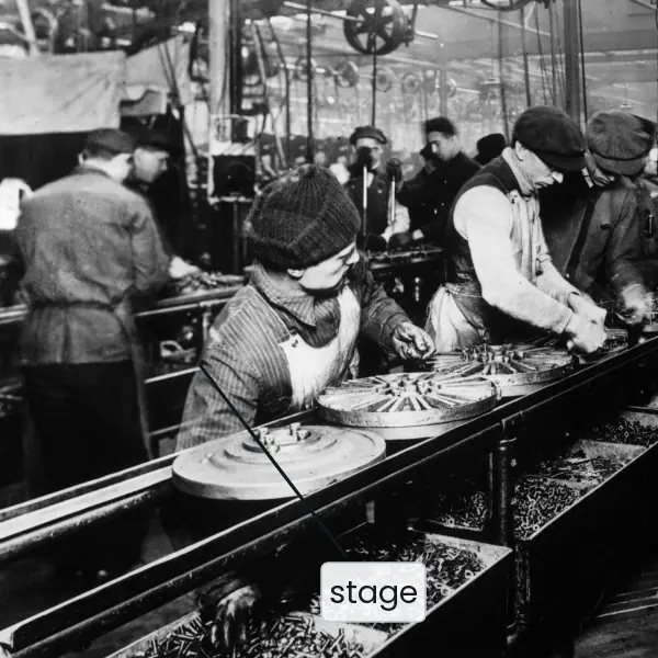
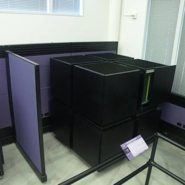
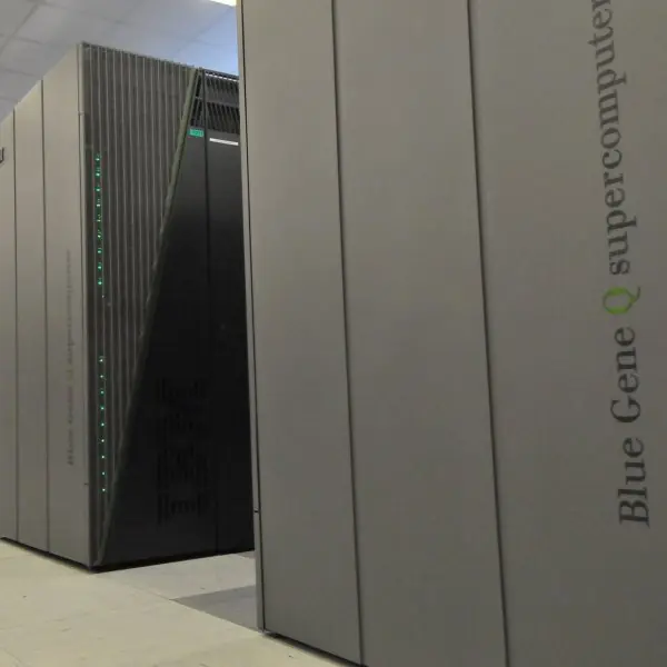
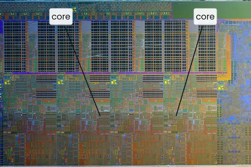
The plate starts with a real assembly line (a pipeline you can see), then shows the real machines that appeared when designers copied the idea in silicon: a vector supercomputer, a data-parallel machine, a many-node cluster, a multi-core die and a crossbar switch.
The figures then draw the timing that the words describe. Every number in them was computed by a short Python program.

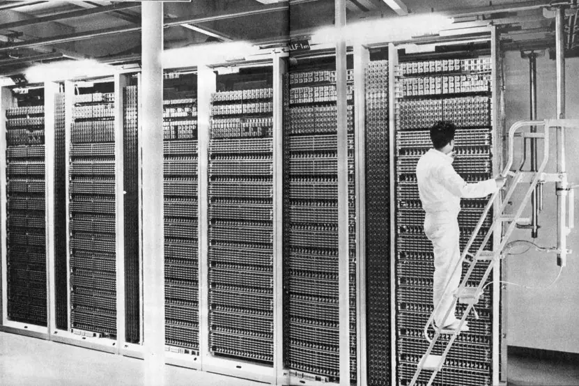


8.8.1 Eight uses of pipelining, vector and parallel processing in Nepal
- Every phone and laptop processor is pipelined. The ARM cores in phones sold in New Road and the Intel or AMD chips in student laptops all overlap fetch, decode, execute and write-back. This is why a processor with a 2 GHz clock can finish close to two billion simple instructions each second. A pipeline is the main reason a cheap phone feels fast.
- Branch prediction in everyday programs. Loops in a Python or Java program written in a TU lab end with a branch that is taken many times and then not taken. The two-bit predictor of Fig. 8.6 guesses this almost always right. Without it the pipeline would waste cycles on every loop and the same program would run noticeably slower.
- GPUs and SIMD instructions for video and games. Decoding a YouTube video, playing an online game or applying a filter in a photo app runs the same operation on thousands of pixels. A GPU or an AVX or NEON instruction does this in lock-step. This is the SIMD class of Flynn's classification, and it is why a small graphics chip can beat a big CPU on pictures.
- Multi-core PCs and servers. A quad-core PC in a college lab can run a browser, an IDE and a video call at the same time, each on its own core. A web server for a school or a university results portal handles many students at once in the same way. This is a MIMD multiprocessor on one chip, as in Plate 8.2.
- Weather and flood modelling. Forecast models, such as those used by the Department of Hydrology and Meteorology and international partners for the Koshi and Narayani basins, divide the land into a grid and apply the same equations to every cell. This vector-style work runs well on clusters and supercomputers. More processors give a faster forecast, up to the limit of Amdahl's law.
- Cloud servers behind payments and e-government. Services such as ConnectIPS, Fonepay and the Nagarik App run on cloud or data-centre servers with many cores. Thousands of users can be served at once because each request runs on a separate core or thread. The cores share memory, so cache coherence (Fig. 8.10) keeps their copies of the data consistent.
- Matrix work in AI and image processing. Face matching for the e-passport, driving-licence or national ID systems, and the machine-learning models taught in BCA, spend most of their time multiplying matrices. This is the vector and systolic-array style of Fig. 8.7. Specialised hardware, such as a GPU, does this work many times faster than a plain CPU loop.
- Telecom and network equipment. The routers and switches in Nepal Telecom, Ncell and ISP networks use multi-core network processors and crossbar-style switching fabrics. Each packet is handled on its own core while others are being forwarded. This lets one box carry the traffic of thousands of customers at the same time.
Formula and fact sheet
- Flynn: SISD, SIMD, MISD, MIMD.
- Pipeline time = (k + n − 1) t_p; speed-up S = n k /(k + n − 1) → k; efficiency = S/k.
- Four-segment instruction pipeline: FI, DA, FO, EX. Hazards: structural, data (RAW/WAR/WAW), control.
- Branch CPI = 1 + (branch fraction) × (taken fraction) × (penalty).
- Matrix multiplication n × n: n³ multiplications, n²(n − 1) additions.
- Amdahl: S = 1/((1 − P) + P/N); limit 1/(1 − P).
Chapter summary
- Flynn classifies computers by instruction and data streams; modern machines are mostly MIMD with SIMD units.
- A k-stage pipeline gives up to k-fold speed-up, reduced by fill time, unbalanced stages and hazards.
- Arithmetic pipelines segment operations like floating-point add; the four-segment instruction pipeline overlaps FI, DA, FO and EX.
- Structural, data and control hazards are handled by resources, forwarding/interlocks and branch prediction.
- Vector processors apply one operation to arrays, removing loop overhead; matrix multiplication is the model workload.
- Multiprocessors share memory over a bus, crossbar or network; caches need coherence protocols; Amdahl's law bounds the gain.
Practice
- Explain Flynn's classification with examples of each class.
- A 5-stage pipeline processes 20 tasks at 5 ns per stage. Find the time, speed-up and efficiency.
- Draw the space–time diagram of a four-segment instruction pipeline for 5 instructions and count the clocks.
- Explain the four-segment floating-point pipeline and trace 0.5 + 0.375.
- Describe structural, data and control hazards and how each is handled.
- Explain operand forwarding with an example.
- List four techniques for handling branch instructions.
- What is vector processing? How many multiplications and additions does a 3 × 3 matrix product need?
- Compare common bus, crossbar and multistage network interconnections.
- What is cache coherence? Compute Amdahl speed-up for P = 0.8, N = 8.
Answers and worked solutions
1. SISD — one CPU on one stream (8085); SIMD — one instruction on many data (GPU, AVX); MISD — many instructions on one data stream (rare, fault-tolerant); MIMD — independent CPUs (multi-core, cluster).
2. Pipelined: (5 + 20 − 1) × 5 = 120 ns; non-pipelined: 20 × 5 × 5 = 500 ns; S = 500/120 = 4.17; efficiency = 4.17/5 = 0.83.
3. I1..I5 in a four-stage pipeline finish at clock 4 + 5 − 1 = 8 (each instruction starts one clock after the previous one).
4. Stages: compare exponents → align mantissas → add/subtract mantissas → normalise. 0.5 = 1.0 × 2⁻¹, 0.375 = 1.1 × 2⁻²; difference 1 → shift 0.375's mantissa right → 0.11 × 2⁻¹; add 1.0 + 0.11 = 1.11 × 2⁻¹ = 0.875.
5. Structural — resource conflict (add resources, separate caches); data — dependency on a pending result (forwarding, interlock, scheduling); control — a branch changes the PC (prediction, delayed branch, BTB).
6. Instead of waiting for ADD R1,R2,R3 to write R1, the ALU output is fed straight back to the ALU input of the next instruction SUB R4,R1,R5, saving the stall cycles.
7. Prefetch both paths, branch target buffer, branch prediction, loop buffer, delayed branch.
8. One instruction operates on whole arrays (e.g. adds two 100-element vectors). 3 × 3: n³ = 27 multiplications and n²(n − 1) = 9 × 2 = 18 additions.
9. Bus: cheapest, one transfer at a time; crossbar: many simultaneous transfers, n² switches; multistage: n log n switches, some blocking.
10. Coherence = keeping the copies of a shared variable in different caches consistent (write-invalidate, snooping/MESI, directory). Amdahl: S = 1/(0.2 + 0.8/8) = 1/0.3 = 3.33.
Model answers for Unit 8
Q1. Explain Flynn's classification of parallel computers with a block diagram and an example of each class. (5 marks)
Michael Flynn classified computers in 1966 by the number of instruction streams (IS) and data streams (DS) that they handle at the same time.
An instruction stream is the sequence of instructions executed by a control unit (CU); a data stream is the sequence of operands handled by a processing unit (PU). Fig. 8.1 draws the four classes.
| Class | Instruction streams | Data streams | Example |
|---|---|---|---|
| SISD | one | one | classic uniprocessor such as the 8085 |
| SIMD | one | many | vector processor, GPU, AVX or NEON instructions, CM-2 |
| MISD | many | one | rare; fault-tolerant flight computers, some systolic arrays |
| MIMD | many | many | multi-core PC, SMP server, cluster, Blue Gene |
In SISD one CU fetches instructions one after another and drives one PU on one stream of data. In SIMD one CU broadcasts the same instruction to many PUs, each working on its own data, so one ADD adds many pairs of numbers.
In MISD several CUs act on the same data stream as it passes along a chain; real examples are few.
In MIMD every processor has its own CU and its own program and data; the processors may share memory (multiprocessor) or have private memory and exchange messages (multicomputer).
A modern PC is MIMD across its cores and SIMD inside each core.
Q2. What is pipelining? Derive the speed-up and efficiency of a k-stage pipeline and explain why the real speed-up is lower. (5 marks)
Pipelining splits a task into k stages separated by registers, each stage taking one clock period t_p. While task 1 is in stage 2, task 2 is already in stage 1, like cars on an assembly line (Plate 8.1). Once the pipeline is full, one task finishes every clock.
For n tasks, the first needs k clocks and every later task needs one more, so the pipelined time is (k + n − 1) t_p (Fig. 8.2: 4 + 6 − 1 = 9 clocks). Without a pipeline the tasks take n k t_p. Therefore
- Speed-up S = n k / (k + n − 1), which tends to k as n becomes large.
- Efficiency = S / k, the fraction of the stages kept busy.
- Throughput = n / ((k + n − 1) t_p), tending to one result per clock.
For k = 4 and n = 100 the speed-up is 400 / 103 = 3.88 and the efficiency 0.97 (Fig. 8.3). For a single task S = 1.
The real speed-up is lower because (1) the pipeline needs k − 1 clocks to fill and drain, (2) stages are not equal in delay and the slowest one sets the clock, (3) registers between stages add delay, and (4) hazards force stalls: structural conflicts, data dependencies and branches.
Q3. A five-stage pipeline with a stage delay of 4 ns executes 30 tasks. Find the time, speed-up, efficiency and throughput. (5 marks)
Given k = 5, n = 30, t_p = 4 ns. The same method applies whatever the numbers are.
Pipelined time. The first task leaves after 5 clocks and the other 29 leave one per clock, so the number of clocks is k + n − 1 = 5 + 29 = 34. The time is 34 × 4 = 136 ns.
Non-pipelined time. Each task passes all five stages one after another, so the time is n k t_p = 30 × 5 × 4 = 600 ns.
Speed-up. S = 600 / 136 = 4.41. This is the same as n k / (k + n − 1) = 150 / 34 = 4.41.
Efficiency. E = S / k = 4.41 / 5 = 0.882, so the stages are busy 88.2% of the time.
Throughput. n / time = 30 / 136 ns = 0.2206 tasks per ns, which is about 220.6 million tasks per second. The non-pipelined machine gives 30 / 600 = 50 million per second.
| Quantity | Pipelined | Not pipelined |
|---|---|---|
| Total time | 136 ns | 600 ns |
| Tasks per second | 220.6 million | 50 million |
| Speed-up | 4.41 | 1 |
If the number of tasks grew to 1000, the speed-up would rise to 5000 / 1004 = 4.98, close to the ideal limit of k = 5. This shows that a pipeline pays off for long, steady streams of work, which is why instruction pipelines are so successful.
Q4. Explain the four-segment floating-point adder pipeline and trace 0.75 + 0.15625 through it. (5 marks)
Floating-point addition cannot simply add the mantissas because the exponents may differ. The operation is split into four segments, with a register between each pair (Fig. 8.4):
- Compare exponents. Subtract them; the larger one becomes the exponent of the result and the difference tells how far to shift.
- Align mantissas. Shift the mantissa of the number with the smaller exponent to the right by the difference.
- Add or subtract the mantissas.
- Normalise the result. Shift it back to the form 1.xxx and adjust the exponent; round if needed.
Trace. X = 0.75 = 1.1 × 2⁻¹ and Y = 0.15625 = 1.01 × 2⁻³ (binary mantissas).
| Segment | Work | Result |
|---|---|---|
| 1 | exponents −1 and −3, difference 2 | exponent −1 kept |
| 2 | shift 1.01 right by 2 places | 0.0101 × 2⁻¹ |
| 3 | 1.1 + 0.0101 | 1.1101 × 2⁻¹ |
| 4 | already in form 1.xxx | 1.1101 × 2⁻¹ |
The result is 1.1101₂ × 2⁻¹ = 1.8125 × 0.5 = 0.90625, which equals 0.75 + 0.15625.
Because the segments are separated by registers, four different additions can be in the four segments at once, so after the pipeline fills a result is produced every clock.
This is how vector processors and floating-point units deliver one sum per cycle.
Q5. Explain the hazards that occur in an instruction pipeline and the methods used to reduce their effect, including branch handling. (10 marks)
A hazard is a condition that prevents the next instruction from executing in its own clock cycle. The pipeline must then stall (insert bubbles) or take another action, and the speed-up falls.
1. Structural hazards occur when two instructions need the same hardware at the same time, for example one memory port used both for fetching an instruction and for loading an operand.
The remedy is to duplicate the resource, such as separate instruction and data caches.
2. Data hazards occur when an instruction needs a result that an earlier one has not produced yet.
| Type | Meaning | Example |
|---|---|---|
| RAW (true dependency) | I2 reads what I1 writes | ADD R1,R2,R3 then SUB R4,R1,R5 |
| WAR (anti-dependency) | I2 writes what I1 reads | arises with out-of-order issue |
| WAW (output dependency) | both write the same register | arises with out-of-order issue |
In the five-stage pipeline of Fig. 8.5 the SUB must wait two cycles for the ADD result to be written.
Remedies are a hardware interlock (stall), operand forwarding (the ALU output is sent straight to the next ALU input, removing the stall), and compiler scheduling (an independent instruction or a NOP is placed in the gap).
A load followed at once by its use still needs one stall.
3. Control (branch) hazards occur because a branch changes the PC after the next instructions have already been fetched. Techniques:
- Prefetch both paths into separate buffers and discard one.
- Branch target buffer (BTB): a small cache holding the target address of recent branches.
- Branch prediction: static (not taken, or backward taken) or dynamic. A two-bit counter (Fig. 8.6) mispredicts a loop once per exit, 90% accuracy for a loop of 10.
- Loop buffer for small loops, and delayed branch, in which the compiler fills the slot after the branch with a useful instruction.
Effect on CPI. With 20% branches and a 2-cycle penalty, stalling on every branch gives CPI = 1 + 0.2 × 2 = 1.40, always-not-taken with 60% taken gives 1.24, and a 90% accurate predictor gives 1 + 0.2 × 0.1 × 2 = 1.04.
In conclusion, pipelines deliver close to one instruction per clock only when hazards are removed by duplicated hardware, forwarding and good prediction.
Q6. What is vector processing? Why does it speed up scientific programs, and how many operations does matrix multiplication need? (5 marks)
Scientific programs, such as weather models, structural analysis and graphics, apply the same operation to long arrays.
A vector processor has instructions that operate on a whole vector, so C(1:64) = A(1:64) + B(1:64) is one instruction instead of a loop of 64 iterations. A Cray-1 had eight vector registers of 64 elements each (Plate 8.1).
The speed-up has several sources:
- Fewer instruction fetches and decodes: one instruction replaces 64 iterations.
- No loop overhead and no branch hazards inside the vector.
- Pipelined arithmetic: after a start-up of 6 clocks, the six-stage adder gives one sum per clock, so 64 additions take 6 + 63 = 69 clocks instead of 64 × 6 = 384, a speed-up of 5.6 (Fig. 8.7).
- Interleaved memory supplies one operand per clock because consecutive addresses lie in different modules.
Matrix multiplication. For n × n matrices, C = A × B needs n³ multiplications and n²(n − 1) additions.
Each element C(i,j) is the inner product of row i of A and column j of B. For n = 2 this is 8 multiplications and 4 additions; for n = 3 it is 27 and 18. With A = [[1,2],[3,4]] and B = [[5,6],[7,8]], C = [[19,22],[43,50]].
Each inner product is a stream of multiply-add operations, so several pipelines can compute different rows at once. Systolic arrays and GPUs use this idea.
Q7. What is a multiprocessor? Describe the interconnection structures and the cache coherence problem and its solutions. (10 marks)
A multiprocessor is a computer with two or more CPUs that share one memory and run under one operating system, a tightly coupled MIMD system. A multicomputer or cluster has separate memories and exchanges messages.
Multiprocessors give higher throughput, speed for parallel programs, graceful degradation if a CPU fails, and the ability to add processors.
Interconnection structures.
| Structure | Idea | Advantage | Limit |
|---|---|---|---|
| Common bus | all CPUs and memories on one bus | cheap and simple | only one transfer at a time |
| Multiport memory | one port per CPU on each memory | high bandwidth | many wires, complex memory |
| Crossbar | a switch at each CPU-memory crossing | many simultaneous transfers | n × n switches (4096 for n = 64) |
| Multistage (Omega) | log₂ n stages of 2 × 2 switches | (n / 2) log₂ n switches (192 for n = 64) | some blocking |
| Hypercube | 2ⁿ nodes, each linked to n neighbours | any node in n hops | wiring grows with n |
Fig. 8.8 shows a crossbar carrying four transfers at once, and Fig. 8.9 a 3-cube in which a message flips one address bit per hop. Arbitration (fixed priority, rotating priority or daisy chain) decides who gets a shared bus.
Cache coherence. Each CPU has a private cache, so two caches may hold different values of the same variable. If CPU A writes X = 7 and CPU B still holds X = 5, B reads stale data. Solutions:
- Write-invalidate: a write removes all other copies; this is the common choice.
- Write-update (broadcast): a write sends the new value to all copies.
- Snooping: each cache watches the shared bus for writes. The MESI protocol labels each line Modified, Exclusive, Shared or Invalid (Fig. 8.10).
- Directory-based: a directory records which caches hold each block, so only those are contacted; it scales to larger systems.
For example, with a shared bus every miss in any cache uses the same wires, so beyond a few cores a bus saturates and designers move to crossbars, rings or directory-based networks, as in server chips with dozens of cores.
Programs also need synchronisation (locks built from atomic test-and-set, semaphores, barriers).
In conclusion, the speed of a multiprocessor depends as much on the interconnect and coherence cost as on the number of CPUs, and Amdahl's law limits what extra CPUs can achieve.
Q8. State Amdahl's law. A program is 95% parallelisable; find the speed-up on 8 and 64 processors and the upper limit. (5 marks)
Amdahl's law says that if a fraction P of a program can be run in parallel on N processors and the rest, 1 − P, must run serially, the speed-up is
S = 1 / ((1 − P) + P / N).
The serial part does not shrink, so it sets a ceiling: as N grows, S tends to 1 / (1 − P).
For P = 0.95:
- N = 8: S = 1 / (0.05 + 0.95 / 8) = 1 / (0.05 + 0.11875) = 1 / 0.16875 = 5.93.
- N = 64: S = 1 / (0.05 + 0.95 / 64) = 1 / (0.05 + 0.01484) = 1 / 0.06484 = 15.4.
- Limit (N → ∞): S = 1 / 0.05 = 20.
| Processors | Speed-up | Efficiency S / N |
|---|---|---|
| 1 | 1.00 | 100% |
| 8 | 5.93 | 74% |
| 64 | 15.4 | 24% |
| unlimited | 20 | → 0% |
The table shows that eight times more processors (from 8 to 64) gives only 2.6 times more speed. Fig. 8.11 compares three programs; a program with P = 0.5 can never run more than twice as fast.
The lesson is that the serial fraction must be reduced as much as the processor count is raised.