Unit 10 · Statistics and Probability · 8 teaching hours · 37 min read
Correlation and Regression
What the syllabus asks for 5
- Correlation and its nature
- Karl Pearson's coefficient of correlation and interpretation
- Properties of correlation coefficient (without proof)
- Rank correlation (elementary concept)
- Regression equations: line of y on x and x on y
Two measurements taken on the same individuals are often related: taller fathers tend to have taller sons, more rainfall tends to mean a bigger maize harvest, a higher price tends to mean fewer kilograms sold. Correlation answers how strongly two such quantities move together and in which direction. Regression goes one step further and gives an equation, so that from a value of one variable we can estimate a value of the other. This unit teaches you to build both from a table of data — by hand, with every column written out.
Nearly every question is one of five shapes: draw or read a scatter diagram, compute Karl Pearson's r from a table, compute Spearman's r_s from ranks, find the two regression lines and estimate, or given the two lines, work backwards to \bar{x}, \bar{y} and r. The marks are in the table — set out your columns and totals neatly, because the examiner follows them line by line.
10.1 Correlation and its nature
Two variables are correlated if a change in one is accompanied by a systematic change in the other. The single number that measures the strength and direction of this joint movement is called a coefficient of correlation.
Correlation is classified in three ways.
By direction.
- Positive correlation — the variables move the same way; x up, y up. Rainfall and crop yield; height and weight.
- Negative correlation — they move in opposite ways; x up, y down. Price of a vegetable and quantity demanded; speed of a bus and time taken.
- Zero (no) correlation — no systematic movement at all. Shoe size and marks in Mathematics.
By form.
- Linear correlation — the points of the scatter diagram cluster about a straight line. The ratio of change is roughly constant.
- Non-linear (curvilinear) correlation — they cluster about a curve. Fertiliser and yield behave like this: yield rises, flattens, then falls.
By number of variables. Correlation between two variables only is simple correlation (all of this unit). With three or more variables, studying all of them together is multiple correlation, and studying two of them while holding the rest fixed is partial correlation.
The scatter diagram
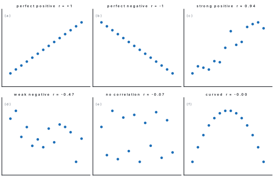
Plot each pair (x, y) as a dot on graph paper. The resulting scatter diagram is the quickest way to judge correlation — before any arithmetic.
- Dots rising from lower-left to upper-right → positive correlation.
- Dots falling from upper-left to lower-right → negative correlation.
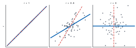
- Dots on one straight line exactly → perfect correlation (r = \pm 1).
- A tight band → strong; a fat cloud → weak; a shapeless blob → zero.
Problem. The table gives the price of tomatoes (Rs per kg) at Kalimati market and the quantity sold (quintal) on five days. Draw a scatter diagram and state the nature of the correlation.
| Price x | 120 | 140 | 160 | 180 | 200 |
|---|---|---|---|---|---|
| Quantity y | 11 | 8 | 9 | 7 | 5 |
Solution. Plot (120, 11), (140, 8), (160, 9), (180, 7), (200, 5) with price on the horizontal axis. As we move right the dots move down, and they lie close to a straight line falling to the right.
Hence the correlation is negative, linear and strong — a rise in price goes with a fall in the quantity sold. (Worked example 10.3 will show r = -0.92, confirming the picture.)
10.2 Karl Pearson's coefficient of correlation and interpretation
Karl Pearson's coefficient measures linear correlation. Write d_x = x - \bar{x} and d_y = y - \bar{y} for the deviations from the means.
Cancelling the \frac{1}{n}'s gives the working formula
The n's cancel, so never mind whether you divide by n or not — just be consistent. Three forms of the same coefficient are used, and choosing the right one saves minutes in the exam.
| Form | Use it when | Formula |
|---|---|---|
| Actual mean | \bar{x}, \bar{y} are whole numbers | r = \dfrac{\sum d_x d_y}{\sqrt{\sum d_x^{2}\sum d_y^{2}}} |
| Raw score (direct) | the numbers are small | r = \dfrac{n\sum xy - \sum x \sum y}{\sqrt{\left[n\sum x^{2} - (\sum x)^{2}\right]\left[n\sum y^{2} - (\sum y)^{2}\right]}} |
| Assumed mean (short-cut) | \bar{x}, \bar{y} are awkward fractions | r = \dfrac{n\sum d_x d_y - \sum d_x \sum d_y}{\sqrt{\left[n\sum d_x^{2} - (\sum d_x)^{2}\right]\left[n\sum d_y^{2} - (\sum d_y)^{2}\right]}} |
In the third row d_x = x - A and d_y = y - B for any convenient assumed means A and B — the answer does not depend on which you pick.
r has no units and always satisfies -1 \le r \le +1.
| |r| | Interpretation |
|---|---|
| 1 | perfect correlation (all points on one line) |
| 0.75 to 1 | high / strong |
| 0.50 to 0.75 | moderate |
| 0.25 to 0.50 | low |
| 0 to 0.25 | very weak, practically none |
The sign carries the direction; the size carries the strength. Also useful: r^{2}, called the coefficient of determination, is the fraction of the variation in y explained by x. So r = 0.8 means 64\% explained.
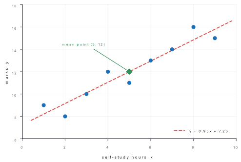
Problem. Nine students report the hours x they spent on self-study in a week and score y marks out of 20 in the test that followed. Compute Karl Pearson's coefficient of correlation.
| x | 1 | 2 | 3 | 4 | 5 | 6 | 7 | 8 | 9 |
|---|---|---|---|---|---|---|---|---|---|
| y | 9 | 8 | 10 | 12 | 11 | 13 | 14 | 16 | 15 |
Solution. The numbers are small, so use the raw-score form. Build the table.
| x | y | xy | x^{2} | y^{2} |
|---|---|---|---|---|
| 1 | 9 | 9 | 1 | 81 |
| 2 | 8 | 16 | 4 | 64 |
| 3 | 10 | 30 | 9 | 100 |
| 4 | 12 | 48 | 16 | 144 |
| 5 | 11 | 55 | 25 | 121 |
| 6 | 13 | 78 | 36 | 169 |
| 7 | 14 | 98 | 49 | 196 |
| 8 | 16 | 128 | 64 | 256 |
| 9 | 15 | 135 | 81 | 225 |
| 45 | 108 | 597 | 285 | 1356 |
So n = 9, \sum x = 45, \sum y = 108, \sum xy = 597, \sum x^{2} = 285, \sum y^{2} = 1356. Substituting,
r = +0.95: a very high positive correlation. Since r^{2} = 0.9025, about 90\% of the variation in marks is explained by study hours.
Problem. Find Karl Pearson's coefficient of correlation for the price and quantity data of Worked example 10.1.
Solution. Here \bar{x} = \dfrac{800}{5} = 160 and \bar{y} = \dfrac{40}{5} = 8 — both whole numbers, so use the actual-mean form with d_x = x - 160, d_y = y - 8.
| x | y | d_x | d_y | d_x d_y | d_x^{2} | d_y^{2} |
|---|---|---|---|---|---|---|
| 120 | 11 | -40 | 3 | -120 | 1600 | 9 |
| 140 | 8 | -20 | 0 | 0 | 400 | 0 |
| 160 | 9 | 0 | 1 | 0 | 0 | 1 |
| 180 | 7 | 20 | -1 | -20 | 400 | 1 |
| 200 | 5 | 40 | -3 | -120 | 1600 | 9 |
| 0 | 0 | -260 | 4000 | 20 |
The two deviation columns must total zero — that is your check. Now substitute:
A high negative correlation: as the price rises, the quantity sold falls.
Short cut. Dividing every d_x by 20 turns the column into -2, -1, 0, 1, 2, and then \sum d_x d_y = -13, \sum d_x^{2} = 10, so
exactly as before. Section 10.3 explains why dividing by 20 changed nothing.
Problem. The heights (in inches) of 8 fathers and their sons are given. Calculate the coefficient of correlation.
| Father x | 65 | 63 | 67 | 64 | 68 | 62 | 70 | 66 |
|---|---|---|---|---|---|---|---|---|
| Son y | 68 | 66 | 68 | 65 | 69 | 66 | 68 | 65 |
Solution. \sum x = 525 and \sum y = 535, so \bar{x} = 65.625 and \bar{y} = 66.875 — fractions. Use the assumed-mean form with A = 66, B = 67, i.e. d_x = x - 66 and d_y = y - 67.
| x | y | d_x | d_y | d_x d_y | d_x^{2} | d_y^{2} |
|---|---|---|---|---|---|---|
| 65 | 68 | -1 | 1 | -1 | 1 | 1 |
| 63 | 66 | -3 | -1 | 3 | 9 | 1 |
| 67 | 68 | 1 | 1 | 1 | 1 | 1 |
| 64 | 65 | -2 | -2 | 4 | 4 | 4 |
| 68 | 69 | 2 | 2 | 4 | 4 | 4 |
| 62 | 66 | -4 | -1 | 4 | 16 | 1 |
| 70 | 68 | 4 | 1 | 4 | 16 | 1 |
| 66 | 65 | 0 | -2 | 0 | 0 | 4 |
| -3 | -1 | 19 | 51 | 17 |
With n = 8,
So r \approx 0.64: a moderate positive correlation between the heights of fathers and sons.
A high r says the two variables move together; it does not prove that one causes the other. Sales of umbrellas and sales of raincoats in Pokhara are highly correlated, but neither causes the other — rainfall causes both. Always add a sentence of interpretation, never a claim of cause.
10.3 Properties of correlation coefficient (without proof)
The syllabus asks you to state and use these; proofs are not required.
- Range. -1 \le r \le +1. A value outside this range means an arithmetic mistake.
- Symmetry. r_{xy} = r_{yx} — it does not matter which variable you call x.
- Unit-free. r is a pure number. Changing inches to centimetres does not change it.
- Independent of change of origin and scale. If u = \dfrac{x - A}{h} and v = \dfrac{y - B}{k} with h, k > 0, then r_{uv} = r_{xy}. This is the licence for every short-cut method. (If exactly one of h, k is negative, the sign of r flips.)
- Perfect correlation. r = \pm 1 if and only if all the points lie exactly on one straight line; r = +1 for a rising line, r = -1 for a falling one.
- Zero correlation. r = 0 means no linear relationship. The variables may still be strongly related in a curved way — see the curved panel of the scatter-diagram figure in §10.1.
- Geometric mean of the regression coefficients. r = \pm\sqrt{b_{yx} \cdot b_{xy}}, and r, b_{yx}, b_{xy} always carry the same sign.
- Coefficient of determination. r^{2} (0 \le r^{2} \le 1) is the proportion of the variance of one variable explained by the other.
Problem. For the data below compute r. Then code the data as u = \dfrac{x - 30}{10} and v = y - 15, compute r_{uv}, and verify property 4.
| x | 10 | 20 | 30 | 40 | 50 |
|---|---|---|---|---|---|
| y | 12 | 15 | 14 | 18 | 21 |
Solution. Original data. \bar{x} = 30, \bar{y} = 16.
| x | y | d_x | d_y | d_x d_y | d_x^{2} | d_y^{2} |
|---|---|---|---|---|---|---|
| 10 | 12 | -20 | -4 | 80 | 400 | 16 |
| 20 | 15 | -10 | -1 | 10 | 100 | 1 |
| 30 | 14 | 0 | -2 | 0 | 0 | 4 |
| 40 | 18 | 10 | 2 | 20 | 100 | 4 |
| 50 | 21 | 20 | 5 | 100 | 400 | 25 |
| 0 | 0 | 210 | 1000 | 50 |
Coded data. u = -2, -1, 0, 1, 2 and v = -3, 0, -1, 3, 6, so \sum u = 0, \sum v = 5, \sum uv = 21, \sum u^{2} = 10, \sum v^{2} = 55, n = 5:
The two values agree exactly: shifting the origin by 30 and 15 and shrinking the scale by 10 left r untouched.
10.4 Rank correlation (elementary concept)
Sometimes the data are not numbers but positions: the order in which eight dancers were placed by a judge, or the order of preference of ten tea samples. Sometimes the numbers exist but are badly skewed by one extreme value. In both cases we replace each value by its rank and correlate the ranks. The result is Spearman's rank correlation coefficient, written r_s (or \rho).
Rank each variable separately from 1 to n, let D be the difference of the two ranks of an individual, and put
Like r, it lies between -1 and +1.
Rules for ranking, in order:
- Rank 1 goes to the largest value (or the smallest — but then do the same for both variables).
- If two or more values are tied, give each of them the average of the ranks they would have occupied. Two items sharing 4th and 5th place both get rank 4.5; three sharing 8th, 9th, 10th all get rank 9.
- \sum D must come to zero. Use it as a check.
When ranks are tied, \sum D^{2} understates the disagreement, so add a correction to it. For every group of m tied values add \dfrac{m^{3}-m}{12}:
A group of 2 contributes \frac{8-2}{12} = 0.5, a group of 3 contributes \frac{27-3}{12} = 2, a group of 4 contributes \frac{64-4}{12} = 5. Groups in x and in y all count.
Problem. Ten students scored the following marks in Mathematics (x) and in Statistics (y). Compute the rank correlation coefficient.
| Student | A | B | C | D | E | F | G | H | I | J |
|---|---|---|---|---|---|---|---|---|---|---|
| x | 76 | 92 | 64 | 84 | 56 | 72 | 88 | 60 | 80 | 68 |
| y | 66 | 95 | 58 | 78 | 70 | 82 | 90 | 74 | 86 | 62 |
Solution. Rank 1 to the highest mark in each subject separately. All the marks are distinct, so no correction is needed.
| Student | x | y | rank R_x | rank R_y | D = R_x - R_y | D^{2} |
|---|---|---|---|---|---|---|
| A | 76 | 66 | 5 | 8 | -3 | 9 |
| B | 92 | 95 | 1 | 1 | 0 | 0 |
| C | 64 | 58 | 8 | 10 | -2 | 4 |
| D | 84 | 78 | 3 | 5 | -2 | 4 |
| E | 56 | 70 | 10 | 7 | 3 | 9 |
| F | 72 | 82 | 6 | 4 | 2 | 4 |
| G | 88 | 90 | 2 | 2 | 0 | 0 |
| H | 60 | 74 | 9 | 6 | 3 | 9 |
| I | 80 | 86 | 4 | 3 | 1 | 1 |
| J | 68 | 62 | 7 | 9 | -2 | 4 |
| 0 | 44 |
\sum D = 0, as required, and \sum D^{2} = 44 with n = 10:
A fairly high positive rank correlation: students good at Mathematics tend to be placed high in Statistics too.
Problem. Two judges ranked eight performers in a Nepali folk-dance competition as shown. Find the rank correlation coefficient and comment on the agreement between the judges.
| Performer | A | B | C | D | E | F | G | H |
|---|---|---|---|---|---|---|---|---|
| Judge X | 4 | 1 | 7 | 2 | 8 | 5 | 3 | 6 |
| Judge Y | 7 | 1 | 6 | 4 | 5 | 8 | 2 | 3 |
Solution. The ranks are already given, so go straight to D.
| Performer | R_X | R_Y | D | D^{2} |
|---|---|---|---|---|
| A | 4 | 7 | -3 | 9 |
| B | 1 | 1 | 0 | 0 |
| C | 7 | 6 | 1 | 1 |
| D | 2 | 4 | -2 | 4 |
| E | 8 | 5 | 3 | 9 |
| F | 5 | 8 | -3 | 9 |
| G | 3 | 2 | 1 | 1 |
| H | 6 | 3 | 3 | 9 |
| 0 | 42 |
With n = 8, n^{3} - n = 512 - 8 = 504:
r_s = 0.5 — the judges agree only moderately. They agree completely about the winner (both rank B first) but disagree sharply about E and F.
Problem. Find Spearman's rank correlation coefficient for the marks below, applying the correction for tied ranks.
| Student | A | B | C | D | E | F | G | H | I | J |
|---|---|---|---|---|---|---|---|---|---|---|
| Economics x | 36 | 45 | 58 | 45 | 62 | 50 | 55 | 68 | 55 | 48 |
| Statistics y | 40 | 52 | 60 | 48 | 62 | 52 | 44 | 58 | 54 | 46 |
Solution. Rank each column from the highest mark down.
Ranking x. In order: 68, 62, 58, 55, 55, 50, 48, 45, 45, 36. The two 55's occupy places 4 and 5, so each gets \frac{4+5}{2} = 4.5; the two 45's occupy places 8 and 9, so each gets 8.5.
Ranking y. In order: 62, 60, 58, 54, 52, 52, 48, 46, 44, 40. The two 52's occupy places 5 and 6, so each gets 5.5.
| Student | x | y | R_x | R_y | D | D^{2} |
|---|---|---|---|---|---|---|
| A | 36 | 40 | 10 | 10 | 0 | 0 |
| B | 45 | 52 | 8.5 | 5.5 | 3 | 9 |
| C | 58 | 60 | 3 | 2 | 1 | 1 |
| D | 45 | 48 | 8.5 | 7 | 1.5 | 2.25 |
| E | 62 | 62 | 2 | 1 | 1 | 1 |
| F | 50 | 52 | 6 | 5.5 | 0.5 | 0.25 |
| G | 55 | 44 | 4.5 | 9 | -4.5 | 20.25 |
| H | 68 | 58 | 1 | 3 | -2 | 4 |
| I | 55 | 54 | 4.5 | 4 | 0.5 | 0.25 |
| J | 48 | 46 | 7 | 8 | -1 | 1 |
| 0 | 39 |
There are three tied groups, each of size m = 2 (the 55's and the 45's in x, the 52's in y), so the correction is
So r_s \approx 0.755, a high positive rank correlation. (Without the correction you would have got 0.764 — slightly too generous.)
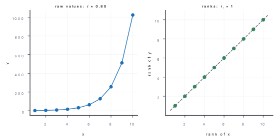
A very common loss of marks: ranking x from the largest and y from the smallest. That reverses the sign of r_s. Decide "rank 1 = highest" and stick to it for both columns. And remember the tie correction — the examiner looks for the \frac{m^{3}-m}{12} term.
10.5 Regression equations: line of y on x and x on y
Correlation stops at a number. Regression fits a line, so that we can estimate. The line of regression of y on x is the straight line that predicts y from x as well as possible; the line of regression of x on y predicts x from y. They are different lines, because "as well as possible" means different things in the two cases.
The method of least squares
For the line of y on x we take the errors vertically: for each point the error is e_i = y_i - (a + bx_i), and we choose a and b to make \sum e_i^{2} as small as possible. (Squares, so that errors above and below the line cannot cancel.)
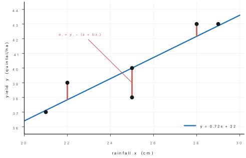
Minimise S = \sum (y_i - a - b x_i)^{2} over a and b. At a minimum both partial derivatives vanish.
Differentiating with respect to a:
Differentiating with respect to b:
Equations (1) and (2) are the normal equations. Dividing (1) by n gives \bar{y} = a + b\bar{x}: the line passes through the mean point (\bar{x}, \bar{y}). Eliminating a between (1) and (2),
This b is called the regression coefficient of y on x and written b_{yx}. Since the line goes through (\bar{x}, \bar{y}) we may write it as
Repeating the whole argument with the roles of x and y exchanged (errors measured horizontally) gives the line of x on y:
Consequences worth memorising:
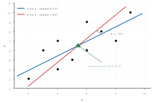
- Both lines pass through (\bar{x}, \bar{y}), so solving them simultaneously gives the two means.
- r^{2} = b_{yx} \cdot b_{xy}, because r\frac{\sigma_y}{\sigma_x} \cdot r\frac{\sigma_x}{\sigma_y} = r^{2}. Hence r = \pm\sqrt{b_{yx}b_{xy}}, with the sign of the b's.
- r, b_{yx} and b_{xy} always have the same sign, and at most one of b_{yx}, b_{xy} can exceed 1 in magnitude (their product is r^2 \le 1).
- If r = \pm 1 the two lines coincide; if r = 0 they are y = \bar{y} and x = \bar{x}, which are perpendicular. The angle between them measures how weak the correlation is:
Problem. The rainfall x (cm) during a growing season and the wheat yield y (quintal per hectare) on six plots in Bhaktapur were:
| x | 21 | 22 | 25 | 25 | 28 | 29 |
|---|---|---|---|---|---|---|
| y | 37 | 39 | 38 | 40 | 43 | 43 |
(a) Find both regression lines. (b) Estimate the yield when the rainfall is 27\ \text{cm}. (c) Find r from the regression coefficients.
Solution. \sum x = 150 so \bar{x} = 25; \sum y = 240 so \bar{y} = 40. Both are whole numbers, so use deviations from the actual means.
| x | y | d_x = x-25 | d_y = y-40 | d_x d_y | d_x^{2} | d_y^{2} |
|---|---|---|---|---|---|---|
| 21 | 37 | -4 | -3 | 12 | 16 | 9 |
| 22 | 39 | -3 | -1 | 3 | 9 | 1 |
| 25 | 38 | 0 | -2 | 0 | 0 | 4 |
| 25 | 40 | 0 | 0 | 0 | 0 | 0 |
| 28 | 43 | 3 | 3 | 9 | 9 | 9 |
| 29 | 43 | 4 | 3 | 12 | 16 | 9 |
| 0 | 0 | 36 | 50 | 32 |
(a) The regression coefficients are
Line of y on x:
Line of x on y:
Check. Put x = 25 in the first: y = 18 + 22 = 40. Put y = 40 in the second: x = 45 - 20 = 25. Both lines pass through (25, 40), as they must.
(b) Yield is being estimated from rainfall, so use the line of y on x:
(c) r^{2} = b_{yx}\,b_{xy} = 0.72 \times 1.125 = 0.81, so r = +\sqrt{0.81} = 0.9 — positive, because both regression coefficients are positive.
Problem. For the self-study data of Worked example 10.2 the totals were n = 9, \sum x = 45, \sum y = 108, \sum xy = 597, \sum x^{2} = 285, \sum y^{2} = 1356. Obtain both regression lines and estimate the marks of a student who studies for 10 hours.
Solution. \bar{x} = \frac{45}{9} = 5 and \bar{y} = \frac{108}{9} = 12. Using the raw-score forms of the regression coefficients,
Hence
For x = 10 hours, y = 0.95(10) + 7.25 = 16.75, so about 17 marks out of 20.
Notice r = \sqrt{0.95 \times 0.95} = 0.95, agreeing with Worked example 10.2. Here b_{yx} = b_{xy} only because \sum d_x^{2} happened to equal \sum d_y^{2}.
To estimate y from a given x, use y on x. To estimate x from a given y, use x on y. Rearranging the wrong line is a standard exam trap and gets zero. Also, a line fitted to rainfall between 21 and 29\ \text{cm} says nothing reliable about 60\ \text{cm} of rain.
Problem. Two regression lines are 4x - 5y + 33 = 0 and 20x - 9y - 107 = 0. Find (a) \bar{x} and \bar{y}, (b) the coefficient of correlation, (c) \sigma_y if the variance of x is 9.
Solution. (a) Both lines pass through (\bar{x}, \bar{y}), so solve them together:
Multiply (1) by 5: \;20x - 25y = -165. Subtract this from (2):
So \bar{x} = 13 and \bar{y} = 17.
(b) Guess that the first line is y on x and the second is x on y:
Since r^{2} = 0.36 \le 1 the guess was right. (Had we got r^{2} > 1 we would simply swap the two lines and try again — that is the whole test.) Both b's are positive, so r = +0.6.
(c) \sigma_x^{2} = 9 gives \sigma_x = 3. From b_{yx} = r\dfrac{\sigma_y}{\sigma_x},
Problem. For a group of 50 students, the mean mark in Mathematics is 36 with standard deviation 11, the mean mark in English is 85 with standard deviation 8, and r = 0.66. Find both regression lines and estimate the English mark of a student who scored 40 in Mathematics.
Solution. Let x be the Mathematics mark and y the English mark, so \bar{x} = 36, \sigma_x = 11, \bar{y} = 85, \sigma_y = 8, r = 0.66.
Line of y on x:
Line of x on y:
For x = 40: \;y = 0.48(40) + 67.72 = 19.2 + 67.72 = 86.92, so about 87 in English.
Check: b_{yx}b_{xy} = 0.48 \times 0.9075 = 0.4356 = (0.66)^{2}. Correct.
Chapter summary
- Correlation measures how two variables move together: positive, negative or zero; linear or curvilinear; simple, multiple or partial. The scatter diagram shows it at a glance.
- Karl Pearson: r = \dfrac{\sum d_x d_y}{\sqrt{\sum d_x^{2}\sum d_y^{2}}} (actual means), or r = \dfrac{n\sum xy - \sum x\sum y}{\sqrt{[n\sum x^{2}-(\sum x)^{2}][n\sum y^{2}-(\sum y)^{2}]}} (raw scores, or deviations from assumed means).
- -1 \le r \le 1; r is symmetric, unit-free and unchanged by a change of origin and scale; r = \pm 1 means all points lie on a line; r = 0 means no linear relation; r^{2} is the fraction of variation explained.
- Spearman: r_s = 1 - \dfrac{6\sum D^{2}}{n^{3}-n}, with \sum D^{2} replaced by \sum D^{2} + \sum\dfrac{m^{3}-m}{12} when ranks are tied. Rank both variables from the same end; check \sum D = 0.
- Least squares gives the normal equations \sum y = na + b\sum x and \sum xy = a\sum x + b\sum x^{2}, whence b_{yx} = \dfrac{\sum d_x d_y}{\sum d_x^{2}} and b_{xy} = \dfrac{\sum d_x d_y}{\sum d_y^{2}}.
- The lines are y - \bar{y} = b_{yx}(x - \bar{x}) and x - \bar{x} = b_{xy}(y - \bar{y}); both pass through (\bar{x}, \bar{y}).
- b_{yx} = r\dfrac{\sigma_y}{\sigma_x}, b_{xy} = r\dfrac{\sigma_x}{\sigma_y}, and r^{2} = b_{yx}\,b_{xy} so r = \pm\sqrt{b_{yx}b_{xy}} with the common sign of the two coefficients.
- Predict y from x with the y-on-x line only; predict x from y with the x-on-y line only.
Practice questions
Group A — Multiple choice (1 mark each)
- The coefficient of correlation always lies between [1]a0 and 1b-1 and +1c-\infty and \inftyd0 and \infty
- If r = 0, the two lines of regression are [1]acoincidentbparallelcperpendiculardinclined at 45^\circ
- If b_{yx} = 0.8 and b_{xy} = 0.45, then r equals [1]a0.36b0.6c0.9d1.25
- For n = 6 pairs of ranks, \sum D^{2} = 14. Spearman's coefficient is [1]a0.4b0.5c0.6d0.8
- Both lines of regression always pass through the point [1]a(0,0)b(\bar{x}, \bar{y})c(\sigma_x, \sigma_y)d(1,1)
- Which value of r is impossible? [1]a-1b-0.98c0d1.04
- A change of origin and scale in x and y (both scales positive) [1]achanges rbleaves r unchangedcchanges the sign of rdmakes r = 0
Answers to Group A
1. (b) — by definition |r| \le 1.
2. (c) — they become y = \bar{y} (horizontal) and x = \bar{x} (vertical).
3. (b) — r = \sqrt{0.8 \times 0.45} = \sqrt{0.36} = 0.6, positive because both b's are positive.
4. (c) — r_s = 1 - \frac{6(14)}{216-6} = 1 - \frac{84}{210} = 0.6.
5. (b) — the normal equation \bar{y} = a + b\bar{x} forces it.
6. (d) — r cannot exceed 1 in magnitude.
7. (b) — property 4 of §10.3; r is independent of origin and scale.
Group B — Short answer (5 marks each)
- Calculate Karl Pearson's coefficient of correlation from the following data. [5]
| x | 2 | 4 | 6 | 8 | 10 |
|---|---|---|---|---|---|
| y | 3 | 7 | 5 | 11 | 14 |
- Ten competitors in a singing contest were ranked by two judges as below. Find the rank correlation coefficient. [5]
| Judge A | 1 | 2 | 3 | 4 | 5 | 6 | 7 | 8 | 9 | 10 |
|---|---|---|---|---|---|---|---|---|---|---|
| Judge B | 2 | 1 | 4 | 5 | 3 | 8 | 6 | 10 | 7 | 9 |
- Find Spearman's rank correlation coefficient, with the correction for ties, for [5]
| x | 50 | 62 | 58 | 50 | 70 | 66 |
|---|---|---|---|---|---|---|
| y | 44 | 52 | 52 | 40 | 60 | 48 |
- Find both lines of regression for the data below and estimate y when x = 6. [5]
| x | 1 | 2 | 3 | 4 | 5 |
|---|---|---|---|---|---|
| y | 2 | 5 | 3 | 8 | 7 |
- The two regression lines of a distribution are 8x - 10y + 66 = 0 and 40x - 18y - 214 = 0. Find \bar{x}, \bar{y} and r. [5]
- For a bivariate distribution, \bar{x} = 18, \bar{y} = 100, \sigma_x = 14, \sigma_y = 20 and r = 0.8. Find the line of regression of y on x and estimate y when x = 25. [5]
- State any five properties of the coefficient of correlation, and explain why a correlation coefficient of 0.9 between two variables does not prove that one causes the other. [5]
Answers to Group B
1. \bar{x} = 6, \bar{y} = 8, so use deviations about the means.
| x | y | d_x | d_y | d_xd_y | d_x^{2} | d_y^{2} |
|---|---|---|---|---|---|---|
| 2 | 3 | -4 | -5 | 20 | 16 | 25 |
| 4 | 7 | -2 | -1 | 2 | 4 | 1 |
| 6 | 5 | 0 | -3 | 0 | 0 | 9 |
| 8 | 11 | 2 | 3 | 6 | 4 | 9 |
| 10 | 14 | 4 | 6 | 24 | 16 | 36 |
| 0 | 0 | 52 | 40 | 80 |
A high positive correlation.
2. D = R_A - R_B gives -1, 1, -1, -1, 2, -2, 1, -2, 2, 1, so D^{2} = 1,1,1,1,4,4,1,4,4,1 and \sum D^{2} = 22 (and \sum D = 0 ✓).
The judges agree closely.
3. Rank each row from the highest. For x: 70, 66, 62, 58, 50, 50 → ranks 1, 2, 3, 4 and the two 50's share places 5 and 6, so each gets 5.5. For y: 60, 52, 52, 48, 44, 40 → the two 52's share places 2 and 3, so each gets 2.5.
| x | y | R_x | R_y | D | D^{2} |
|---|---|---|---|---|---|
| 50 | 44 | 5.5 | 5 | 0.5 | 0.25 |
| 62 | 52 | 3 | 2.5 | 0.5 | 0.25 |
| 58 | 52 | 4 | 2.5 | 1.5 | 2.25 |
| 50 | 40 | 5.5 | 6 | -0.5 | 0.25 |
| 70 | 60 | 1 | 1 | 0 | 0 |
| 66 | 48 | 2 | 4 | -2 | 4 |
| 0 | 7 |
Two tied groups, each of size m = 2, so the correction is 2 \times \frac{2^{3}-2}{12} = 1. With n = 6, n^{3}-n = 210:
4. \bar{x} = 3, \bar{y} = 5.
| x | y | d_x | d_y | d_xd_y | d_x^{2} | d_y^{2} |
|---|---|---|---|---|---|---|
| 1 | 2 | -2 | -3 | 6 | 4 | 9 |
| 2 | 5 | -1 | 0 | 0 | 1 | 0 |
| 3 | 3 | 0 | -2 | 0 | 0 | 4 |
| 4 | 8 | 1 | 3 | 3 | 1 | 9 |
| 5 | 7 | 2 | 2 | 4 | 4 | 4 |
| 0 | 0 | 13 | 10 | 26 |
b_{yx} = \frac{13}{10} = 1.3 and b_{xy} = \frac{13}{26} = 0.5, so
At x = 6: \;y = 1.3(6) + 1.1 = 8.9. (As a bonus, r = \sqrt{1.3 \times 0.5} = \sqrt{0.65} = 0.806.)
5. Solve 8x - 10y = -66 and 40x - 18y = 214 simultaneously. Multiplying the first by 5: 40x - 50y = -330; subtracting from the second gives 32y = 544, so \bar{y} = 17, and then 8x = 10(17) - 66 = 104, so \bar{x} = 13.
Taking the first line as y on x: b_{yx} = \frac{8}{10} = 0.8. Taking the second as x on y: b_{xy} = \frac{18}{40} = 0.45. Then r^{2} = 0.36 \le 1, so the assignment is correct and r = +0.6.
6. b_{yx} = r\dfrac{\sigma_y}{\sigma_x} = 0.8 \times \dfrac{20}{14} = \dfrac{8}{7} = 1.143. Hence
At x = 25: \;y = 1.143(25) + 79.43 = 28.57 + 79.43 = 108.
7. Any five of: -1 \le r \le 1; r_{xy} = r_{yx}; r is a pure number with no units; r is unchanged by a change of origin and scale (sign flips if exactly one scale is negative); r = \pm1 exactly when all points are collinear; r = 0 means no linear relation; r = \pm\sqrt{b_{yx}b_{xy}} and shares the sign of the regression coefficients; r^{2} is the proportion of variation explained.
Causation: a high r only records joint movement. It may arise because x causes y, because y causes x, because a third variable causes both (ice cream sales and drowning deaths both rise with summer heat), or by pure chance in a small sample. Establishing cause needs a controlled experiment or a theory, not a coefficient.
Group C — Long answer (8 marks each)
- (a) What is a scatter diagram? Sketch the scatter diagrams of perfect positive, perfect negative, moderate positive and zero correlation. [3](b) Calculate Karl Pearson's coefficient of correlation for the following data and interpret it. [5]
| x | 2 | 3 | 5 | 7 | 9 | 10 |
|---|---|---|---|---|---|---|
| y | 6 | 5 | 8 | 11 | 12 | 12 |
- (a) Using the method of least squares, derive the equation of the line of regression of y on x and show that it passes through (\bar{x}, \bar{y}). [4](b) Show that r^{2} = b_{yx} \cdot b_{xy}. Hence, if b_{yx} = 0.72 and b_{xy} = 1.125, find r, and find \sigma_y given \sigma_x = 2.89. [4]
- (a) The following table gives the marks of eight students in Accountancy and Economics. Compute Spearman's rank correlation coefficient. [4]
| Accountancy | 68 | 72 | 60 | 84 | 56 | 76 | 64 | 80 |
|---|---|---|---|---|---|---|---|---|
| Economics | 62 | 70 | 68 | 76 | 58 | 80 | 60 | 72 |
(b) For the same data, state which of Pearson's r and Spearman's r_s you would report if one student's Accountancy mark were mis-recorded as 560, and why. [4]
Answers to Group C
1. (a) A scatter diagram plots each pair (x,y) as a dot on rectangular axes; the shape of the cloud shows the nature of the correlation. Perfect positive: all dots on one rising line. Perfect negative: all dots on one falling line. Moderate positive: a fairly wide band rising to the right. Zero: a shapeless cloud with no direction. (See the six panels in §10.1.)
(b) \sum x = 36 so \bar{x} = 6; \sum y = 54 so \bar{y} = 9.
| x | y | d_x | d_y | d_xd_y | d_x^{2} | d_y^{2} |
|---|---|---|---|---|---|---|
| 2 | 6 | -4 | -3 | 12 | 16 | 9 |
| 3 | 5 | -3 | -4 | 12 | 9 | 16 |
| 5 | 8 | -1 | -1 | 1 | 1 | 1 |
| 7 | 11 | 1 | 2 | 2 | 1 | 4 |
| 9 | 12 | 3 | 3 | 9 | 9 | 9 |
| 10 | 12 | 4 | 3 | 12 | 16 | 9 |
| 0 | 0 | 48 | 52 | 48 |
A very high positive correlation: the two variables move up together almost linearly.
2. (a) Let the line be y = a + bx. The vertical error at the i^{\text{th}} point is y_i - a - bx_i, so we minimise S = \sum(y_i - a - bx_i)^{2}. Setting \frac{\partial S}{\partial a} = 0 gives \sum y = na + b\sum x, and \frac{\partial S}{\partial b} = 0 gives \sum xy = a\sum x + b\sum x^{2}. Dividing the first normal equation by n gives \bar{y} = a + b\bar{x}, i.e. the point (\bar{x}, \bar{y}) satisfies the equation, so the line passes through it. Eliminating a between the two normal equations,
and the line may therefore be written y - \bar{y} = b_{yx}(x - \bar{x}).
(b) Since b_{yx} = r\dfrac{\sigma_y}{\sigma_x} and b_{xy} = r\dfrac{\sigma_x}{\sigma_y},
so r = \pm\sqrt{b_{yx}b_{xy}}, the sign being that of the two coefficients. With b_{yx} = 0.72 and b_{xy} = 1.125: r = \sqrt{0.81} = 0.9 (positive).
For \sigma_y: from b_{yx} = r\dfrac{\sigma_y}{\sigma_x},
3. (a) Rank 1 = highest mark in each subject; all marks are distinct.
| Acc. | Eco. | R_x | R_y | D | D^{2} |
|---|---|---|---|---|---|
| 68 | 62 | 5 | 6 | -1 | 1 |
| 72 | 70 | 4 | 4 | 0 | 0 |
| 60 | 68 | 7 | 5 | 2 | 4 |
| 84 | 76 | 1 | 2 | -1 | 1 |
| 56 | 58 | 8 | 8 | 0 | 0 |
| 76 | 80 | 3 | 1 | 2 | 4 |
| 64 | 60 | 6 | 7 | -1 | 1 |
| 80 | 72 | 2 | 3 | -1 | 1 |
| 0 | 12 |
A high positive rank correlation.
(b) Report Spearman's r_s. A single absurd value such as 560 changes the deviations d_x enormously and so drags Pearson's r far from its true value, because r uses the sizes of the observations. Ranking, however, only asks which is biggest: the mis-recorded 560 still ranks first, exactly as 84 did, so r_s is unchanged at 0.857. Rank correlation is the robust choice whenever the data contain an extreme value or come from subjective judgements.
Practise more: Mathematics question bank