Unit 15 · Statistics and Probability · 6 teaching hours · 21 min read
Measures of Dispersion
What the syllabus asks for 3
- Standard deviation and variance
- Coefficient of variation
- Skewness; Karl Pearson's coefficient of skewness
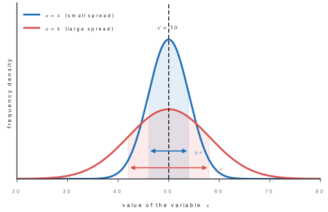
An average tells you where a set of data sits, but nothing about how tightly the values cluster round that centre. Two classes can have the same mean mark of 50 and yet one class may have everyone between 45 and 55 while the other has marks from 5 to 95. Dispersion is the measure of that spread, and it is what turns a single average into a usable description of the data.
Two distributions can share a mean and be completely different. Dispersion measures how far the observations wander from the mean; the standard deviation measures it in the original units, the coefficient of variation measures it as a percentage so that different units can be compared, and skewness measures whether the wandering is symmetric or lopsided.
15.1 Standard deviation and variance
The measures of dispersion, in order of usefulness
| Measure | Formula | Comment |
|---|---|---|
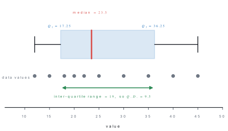
| Range | R = L - S (largest - smallest) | uses only two values; very crude |
| Quartile deviation | Q.D. = \dfrac{Q_3 - Q_1}{2} | ignores the extreme quarter at each end |
| Mean deviation | M.D. = \dfrac{\sum | x - \bar{x}|}{n} | uses all values, but |\ | is awkward algebra |
| Standard deviation | \sigma = \sqrt{\dfrac{\sum (x-\bar{x})^{2}}{n}} | uses all values; the standard measure |
The first three are quick but throw information away. The standard deviation squares the deviations instead of taking their absolute value: squaring removes the sign, keeps every observation in play, and behaves well algebraically. That is why it is the measure used everywhere.
Variance and standard deviation of an individual series
For n observations x_1, x_2, \ldots, x_n with mean \bar{x}, the variance is the mean of the squared deviations and the standard deviation is its positive square root:
Variance is measured in the square of the original unit; standard deviation is in the original unit.
Expanding the square gives a second form that avoids computing every deviation:
and if the mean is awkward, subtract a convenient assumed mean A and work with d = x - A:
Problem. Find the range, mean deviation from the mean, variance and standard deviation of 2, 4, 4, 4, 5, 5, 7, 9.
Solution. Here n = 8 and \sum x = 2+4+4+4+5+5+7+9 = 40, so \bar{x} = 40/8 = 5.
| x | d = x-\bar{x} | | d| | d^{2} |
|---|---|---|---|
| 2 | -3 | 3 | 9 |
| 4 | -1 | 1 | 1 |
| 4 | -1 | 1 | 1 |
| 4 | -1 | 1 | 1 |
| 5 | 0 | 0 | 0 |
| 5 | 0 | 0 | 0 |
| 7 | 2 | 2 | 4 |
| 9 | 4 | 4 | 16 |
| \sum x = 40 | \sum d = 0 | \sum| d| = 12 | \sum d^{2} = 32 |
Range = 9 - 2 = 7.
Check by the \sum x^{2} method. \sum x^{2} = 4+16+16+16+25+25+49+81 = 232, so
The deviations from the mean always add to zero — that is what "mean" means. So \sum d can never be used as a measure of spread, and this is exactly why we square the deviations. Use the \sum d = 0 row as a check on your arithmetic.
Problem. The daily earnings (in hundreds of rupees) of five shopkeepers in Asan bazaar are 25, 32, 43, 19, 21. Find the variance and the standard deviation.
Solution. The mean is not a round number here, so use the \sum x^{2} form.
| x | 25 | 32 | 43 | 19 | 21 | total |
|---|---|---|---|---|---|---|
| x^{2} | 625 | 1024 | 1849 | 361 | 441 | \sum x^{2} = 4300 |
\sum x = 140, n = 5, so \bar{x} = 140/5 = 28.
Discrete frequency distribution
When each value x occurs f times, every sum is weighted by the frequency. With N = \sum f,
Problem. Find the mean, variance and standard deviation of the following distribution.
| Marks (x) | 2 | 4 | 6 | 8 | 10 |
|---|---|---|---|---|---|
| No. of students (f) | 1 | 4 | 6 | 4 | 1 |
Solution. Build the table column by column.
| x | f | fx | d = x - 6 | d^{2} | fd^{2} |
|---|---|---|---|---|---|
| 2 | 1 | 2 | -4 | 16 | 16 |
| 4 | 4 | 16 | -2 | 4 | 16 |
| 6 | 6 | 36 | 0 | 0 | 0 |
| 8 | 4 | 32 | 2 | 4 | 16 |
| 10 | 1 | 10 | 4 | 16 | 16 |
| Total | N=16 | \sum fx = 96 | \sum fd^{2} = 64 |
(The d column was written using this mean, which is why it was computed first.)
Continuous distribution: the step-deviation method
For a grouped distribution take x to be the mid-value of each class. If the class width h is constant, choose an assumed mean A (a convenient mid-value) and set
Then the step-deviation formulae are
These are the fastest hand methods for grouped data. The h multiplies the standard deviation but only the correction term of the mean.
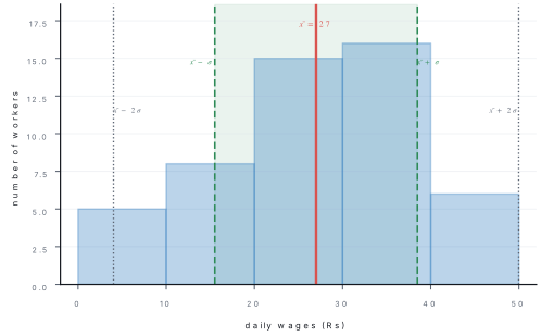
Problem. Calculate the mean and the standard deviation of the following distribution of daily wages.
| Wages (Rs) | 0–10 | 10–20 | 20–30 | 30–40 | 40–50 |
|---|---|---|---|---|---|
| No. of workers | 5 | 8 | 15 | 16 | 6 |
Solution. Take A = 25 (the mid-value of 20–30) and h = 10.
| Class | f | mid x | d' = \dfrac{x-25}{10} | fd' | fd'^{2} |
|---|---|---|---|---|---|
| 0–10 | 5 | 5 | -2 | -10 | 20 |
| 10–20 | 8 | 15 | -1 | -8 | 8 |
| 20–30 | 15 | 25 | 0 | 0 | 0 |
| 30–40 | 16 | 35 | 1 | 16 | 16 |
| 40–50 | 6 | 45 | 2 | 12 | 24 |
| Total | N = 50 | \sum fd' = 10 | \sum fd'^{2} = 68 |
Variance = \sigma^{2} = 132 (rupees squared).
Properties of the standard deviation
- \sigma \geq 0, and \sigma = 0 only when every observation is equal.
- Independent of change of origin. Adding a constant c to every observation leaves \sigma unchanged (the whole distribution shifts, the spread does not).
- Not independent of change of scale. Multiplying every observation by k multiplies \sigma by | k| and the variance by k^{2}.
- Combined standard deviation of two groups with sizes n_1, n_2, means \bar{x}_1, \bar{x}_2 and standard deviations \sigma_1, \sigma_2:
where d_1 = \bar{x}_1 - \bar{x}_{12}, d_2 = \bar{x}_2 - \bar{x}_{12} and \bar{x}_{12} = \dfrac{n_1\bar{x}_1 + n_2\bar{x}_2}{n_1+n_2}.
Problem. The standard deviation of 2, 4, 6, 8, 10 is 2\sqrt{2}. Without recomputing from scratch, write down the standard deviation of (a) 7, 9, 11, 13, 15 and (b) 6, 12, 18, 24, 30.
Solution.
(a) Each value is 5 more than the original: this is a change of origin only. The standard deviation is unchanged, \sigma = 2\sqrt{2} = 2.83.
(b) Each value is 3 times the original: this is a change of scale with k = 3. Hence \sigma' = 3 \times 2\sqrt{2} = 6\sqrt{2} = 8.49, and the variance becomes 9 \times 8 = 72.
Problem. Section A has 50 students with mean mark 54 and \sigma_1 = 8; section B has 100 students with mean mark 60 and \sigma_2 = 10. Find the combined mean and the combined standard deviation.
Solution. Combined mean first:
Deviations of the group means from the combined mean: d_1 = 54 - 58 = -4 and d_2 = 60 - 58 = 2.
15.2 Coefficient of variation
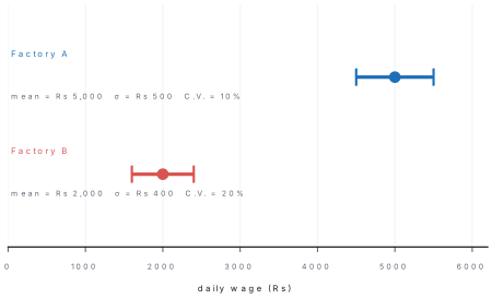
Standard deviation carries the unit of the data, so it cannot compare a distribution of weights in kilograms with one of wages in rupees — and even in the same unit, a standard deviation of Rs 500 means something very different on a mean wage of Rs 5{,}000 than on a mean wage of Rs 2{,}000. Dividing by the mean removes both problems.
It is a pure number (a percentage), independent of the unit of measurement. The series with the greater C.V. is the more variable (less consistent, less uniform, less stable); the series with the smaller C.V. is the more consistent.
Problem. The runs scored by two batsmen in five innings are
| Anil | 44 | 48 | 50 | 52 | 56 |
|---|---|---|---|---|---|
| Bikash | 38 | 46 | 50 | 54 | 62 |
Who is the better scorer on average, and who is the more consistent?
Solution. Both totals are 250, so both means are \bar{x} = 250/5 = 50 runs: on average the two are equally good. Now the deviations.
| Anil x | d = x-50 | d^{2} | Bikash y | d = y-50 | d^{2} | |
|---|---|---|---|---|---|---|
| 44 | -6 | 36 | 38 | -12 | 144 | |
| 48 | -2 | 4 | 46 | -4 | 16 | |
| 50 | 0 | 0 | 50 | 0 | 0 | |
| 52 | 2 | 4 | 54 | 4 | 16 | |
| 56 | 6 | 36 | 62 | 12 | 144 | |
| 250 | 0 | 80 | 250 | 0 | 320 |
Both average 50 runs, but Anil's C.V. is the smaller, so Anil is the more consistent batsman. Bikash is twice as variable.
Problem. Factory A pays a mean daily wage of Rs 5000 with \sigma = Rs 500; factory B pays a mean of Rs 2000 with \sigma = Rs 400. (a) Which factory has more variable wages? (b) If a third factory has C.V. = 25\% and mean wage Rs 4000, find its standard deviation.
Solution.
(a) Compare the coefficients of variation, not the standard deviations:
Factory B has the larger C.V., so B has the more variable wages — even though its standard deviation is the smaller of the two.
(b) Rearranging C.V. = \dfrac{\sigma}{\bar{x}}\times100:
"Series A has \sigma = 500 and series B has \sigma = 400, so B is more consistent" is wrong unless the two means are equal. Consistency questions are always decided by the C.V.
15.3 Skewness; Karl Pearson's coefficient of skewness
Dispersion says how wide a distribution is. Skewness says whether it is lopsided.
A distribution is symmetric if the two halves about the centre are mirror images; then mean = median = mode. It is positively skewed if it has a long tail to the right (mean > median > mode) and negatively skewed if it has a long tail to the left (mean < median < mode).
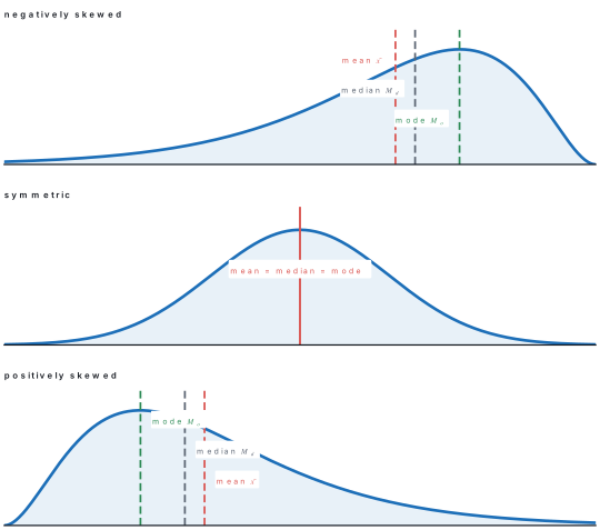
The standard numerical measure is due to Karl Pearson. It measures how far the mean has been dragged from the mode, in units of standard deviation, so the answer is a pure number.
where M_o is the mode. When the mode is ill-defined, use the empirical relation M_o = 3M_d - 2\bar{x} (with M_d the median) to get the second form:
Interpretation: S_k > 0 positively skewed, S_k < 0 negatively skewed, S_k = 0 symmetric. In practice S_k lies between -3 and +3.
Problem. For a distribution, mean = 45, mode = 42 and \sigma = 6. Find Karl Pearson's coefficient of skewness and state the type of skewness.
Solution.
S_k is positive, so the distribution is positively skewed: it has a longer tail on the right-hand (higher-value) side.
Problem. A distribution has mean 50, median 48 and standard deviation 12. Find its coefficient of skewness, and estimate the mode.
Solution. The mode is not given, so use the median form:
From the empirical relation,
and as a check \dfrac{\bar{x}-M_o}{\sigma} = \dfrac{50-44}{12} = 0.5 ✔. The distribution is positively skewed.
Problem. Compute the mean, mode, standard deviation and Karl Pearson's coefficient of skewness for
| Number of absences (x) | 1 | 2 | 3 | 4 | 5 |
|---|---|---|---|---|---|
| Number of students (f) | 10 | 8 | 5 | 4 | 3 |
Solution. Work in one table, including a cumulative-frequency column so the median is available too.
| x | f | c.f. | fx | x^{2} | fx^{2} |
|---|---|---|---|---|---|
| 1 | 10 | 10 | 10 | 1 | 10 |
| 2 | 8 | 18 | 16 | 4 | 32 |
| 3 | 5 | 23 | 15 | 9 | 45 |
| 4 | 4 | 27 | 16 | 16 | 64 |
| 5 | 3 | 30 | 15 | 25 | 75 |
| Total | N = 30 | \sum fx = 72 | \sum fx^{2} = 226 |
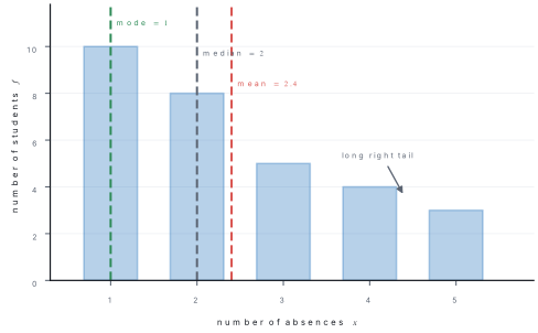
The mode is the value with the largest frequency: M_o = 1 (frequency 10).
The distribution is strongly positively skewed — most students are absent once or twice, with a thin tail of frequent absentees pulling the mean up.
Cross-check with the median. The median is the \left(\frac{N+1}{2}\right)th = 15.5th value; the cumulative frequency reaches 18 at x = 2, so M_d = 2. Then S_k = \dfrac{3(2.4-2)}{1.3317} = 0.90 — the same sign and the same message. The two formulas agree exactly only when the empirical relation M_o = 3M_d - 2\bar{x} holds exactly; here it gives M_o = 6 - 4.8 = 1.2 against the true mode of 1.
Chapter summary
- Dispersion measures spread about the average. Range = L-S; Q.D. = \frac{Q_3-Q_1}{2}; M.D. = \frac{\sum| x-\bar{x}|}{n}.
- Variance \sigma^{2} = \dfrac{\sum(x-\bar{x})^{2}}{n} = \dfrac{\sum x^{2}}{n} - \bar{x}^{2}; standard deviation \sigma = \sqrt{\sigma^{2}}, in the original unit.
- Frequency data: \bar{x} = \dfrac{\sum fx}{N} and \sigma = \sqrt{\dfrac{\sum fx^{2}}{N} - \bar{x}^{2}} with N = \sum f.
- Grouped data (step deviation, d' = \frac{x-A}{h}): \bar{x} = A + \dfrac{\sum fd'}{N}h and \sigma = h\sqrt{\dfrac{\sum fd'^{2}}{N} - \left(\dfrac{\sum fd'}{N}\right)^{2}}.
- \sigma is unchanged by adding a constant and multiplied by | k| when every value is multiplied by k.
- Combined SD: \sigma_{12} = \sqrt{\dfrac{n_1(\sigma_1^{2}+d_1^{2}) + n_2(\sigma_2^{2}+d_2^{2})}{n_1+n_2}} with d_i = \bar{x}_i - \bar{x}_{12}.
- C.V. = \dfrac{\sigma}{\bar{x}}\times100\%: smaller C.V. = more consistent. Use it whenever the means or the units differ.
- Skewness measures lopsidedness: S_k = \dfrac{\bar{x}-M_o}{\sigma} = \dfrac{3(\bar{x}-M_d)}{\sigma}, with M_o = 3M_d - 2\bar{x} as the empirical link.
Practice questions
Group A — Multiple choice (1 mark each)
- The variance is the square of the [1]amean deviationbstandard deviationcquartile deviationdrange
- Standard deviation is independent of change of [1]aoriginbscalecboth origin and scaledneither
- If every observation of a series is multiplied by 4, the standard deviation is [1]aunchangedbmultiplied by 2cmultiplied by 4dmultiplied by 16
- For a symmetric distribution, Karl Pearson's coefficient of skewness is [1]a1b0c-1d3
- Of two series with the same mean, the more consistent is the one with the [1]agreater rangebgreater C.V.csmaller C.V.dgreater variance
- If mean = 30, median = 28 and \sigma = 6, then S_k equals [1]a0.33b1.00c0.67d2.00
Answers to Group A
1. (b) — by definition \sigma^{2} is the variance.
2. (a) — shifting every value leaves all deviations x-\bar{x} unchanged.
3. (c) — \sigma scales with | k|; the variance would become 16 times.
4. (b) — mean = mode, so the numerator \bar{x}-M_o is zero.
5. (c) — a smaller C.V. means less relative variation.
6. (b) — S_k = 3(30-28)/6 = 1.
Group B — Short answer (5 marks each)
- Define variance and standard deviation. Find the standard deviation of 2, 4, 6, 8, 10, 12, 14. [5]
-
Calculate the mean and the standard deviation of the distribution below. [5]
x 5 10 15 20 25 f 1 4 6 4 1 -
Find the mean, standard deviation and coefficient of variation of the following grouped data using the step-deviation method. [5]
Class 0–10 10–20 20–30 30–40 40–50 f 4 6 10 12 8 -
The mean and standard deviation of the heights of the boys in a class are 160 cm and 8 cm; for the girls they are 150 cm and 6 cm. State with reasons which group is more variable in height. [5]
- For a distribution the mean is 40, the median is 38 and the standard deviation is 10. Find the mode and Karl Pearson's coefficient of skewness by both formulae. [5]
- A group of 30 students has mean weight 20 kg with \sigma_1 = 3 kg; another group of 20 students has mean weight 25 kg with \sigma_2 = 4 kg. Find the combined mean and the combined standard deviation. [5]
Answers to Group B
1. Variance is the mean of the squared deviations from the mean; \sigma is its positive square root. Here n = 7, \sum x = 56, so \bar{x} = 8.
| x | 2 | 4 | 6 | 8 | 10 | 12 | 14 | total |
|---|---|---|---|---|---|---|---|---|
| d = x-8 | -6 | -4 | -2 | 0 | 2 | 4 | 6 | 0 |
| d^{2} | 36 | 16 | 4 | 0 | 4 | 16 | 36 | 112 |
\sigma^{2} = 112/7 = 16, so \sigma = 4.
2. N = 16; \sum fx = 5+40+90+80+25 = 240, so \bar{x} = 240/16 = 15. With d = x-15: fd^{2} = 1(100)+4(25)+6(0)+4(25)+1(100) = 400. Hence \sigma^{2} = 400/16 = 25 and \sigma = 5.
3. Mid-values 5,15,25,35,45; take A = 25, h = 10, N = 40.
| x | 5 | 15 | 25 | 35 | 45 | total |
|---|---|---|---|---|---|---|
| f | 4 | 6 | 10 | 12 | 8 | 40 |
| d' | -2 | -1 | 0 | 1 | 2 | |
| fd' | -8 | -6 | 0 | 12 | 16 | 14 |
| fd'^{2} | 16 | 6 | 0 | 12 | 32 | 66 |
\bar{x} = 25 + \frac{14}{40}(10) = 25 + 3.5 = 28.5; \sigma = 10\sqrt{\frac{66}{40} - \left(\frac{14}{40}\right)^{2}} = 10\sqrt{1.65-0.1225} = 10\sqrt{1.5275} = 12.36; and C.V. = \frac{12.36}{28.5}\times100 = 43.37\%.
4. The means differ, so compare coefficients of variation: C.V._{\text{boys}} = \frac{8}{160}\times100 = 5\% and C.V._{\text{girls}} = \frac{6}{150}\times100 = 4\%. The boys' C.V. is larger, so the boys are more variable in height, even though a quick glance at the standard deviations only says their spread is larger in absolute centimetres.
5. M_o = 3M_d - 2\bar{x} = 3(38) - 2(40) = 114 - 80 = 34. Then S_k = \frac{\bar{x}-M_o}{\sigma} = \frac{40-34}{10} = 0.6, and by the median form S_k = \frac{3(40-38)}{10} = 0.6 — the two agree. Positively skewed.
6. \bar{x}_{12} = \frac{30(20)+20(25)}{50} = \frac{600+500}{50} = 22 kg. Then d_1 = 20-22 = -2 and d_2 = 25-22 = 3, so
giving \sigma_{12} = \sqrt{17.8} = 4.22 kg.
Group C — Long answer (8 marks each)
-
(a) Define standard deviation and coefficient of variation, and explain why the coefficient of variation is needed. [2](b) Calculate the mean, standard deviation and coefficient of variation of the marks below. [6]
Marks 0–10 10–20 20–30 30–40 40–50 No. of students 5 10 20 10 5 -
(a) Define skewness and state Karl Pearson's coefficient of skewness in both its forms, explaining how to read its sign. [3](b) Find the mean, mode, standard deviation and coefficient of skewness of the distribution below. [5]
x 10 20 30 40 50 f 2 5 12 8 3
Answers to Group C
1. (a) \sigma = \sqrt{\sum(x-\bar{x})^{2}/n} measures absolute spread in the unit of the data; C.V. = (\sigma/\bar{x})\times100\% measures it as a percentage of the mean. The C.V. is needed because a standard deviation of, say, 500 is large on a mean of 1000 but small on a mean of 50\,000, and because two series in different units cannot otherwise be compared.
(b) Mid-values 5,15,25,35,45; A = 25, h = 10, N = 50.
| x | 5 | 15 | 25 | 35 | 45 | total |
|---|---|---|---|---|---|---|
| f | 5 | 10 | 20 | 10 | 5 | 50 |
| d' | -2 | -1 | 0 | 1 | 2 | |
| fd' | -10 | -10 | 0 | 10 | 10 | 0 |
| fd'^{2} | 20 | 10 | 0 | 10 | 20 | 60 |
\bar{x} = 25 + \frac{0}{50}(10) = 25 marks (the distribution is symmetric).
\sigma = 10\sqrt{\frac{60}{50} - 0^{2}} = 10\sqrt{1.2} = 10(1.0954) = 10.95 marks.
C.V. = \frac{10.95}{25}\times100 = 43.82\%.
2. (a) Skewness is the lack of symmetry of a distribution. Karl Pearson's coefficient is S_k = \dfrac{\bar{x}-M_o}{\sigma}, or S_k = \dfrac{3(\bar{x}-M_d)}{\sigma} when the mode is ill-defined. A positive value means a longer tail to the right, a negative value a longer tail to the left, and zero means symmetry.
(b)
| x | f | fx | x^{2} | fx^{2} |
|---|---|---|---|---|
| 10 | 2 | 20 | 100 | 200 |
| 20 | 5 | 100 | 400 | 2000 |
| 30 | 12 | 360 | 900 | 10800 |
| 40 | 8 | 320 | 1600 | 12800 |
| 50 | 3 | 150 | 2500 | 7500 |
| Total | 30 | 950 | 33300 |
\bar{x} = \frac{950}{30} = 31.67; mode M_o = 30 (largest frequency, 12).
\sigma^{2} = \frac{33300}{30} - (31.67)^{2} = 1110 - 1002.78 = 107.22, so \sigma = 10.35.
S_k = \frac{31.67-30}{10.35} = 0.16: a slight positive skew.
Practise more: Mathematics question bank