Unit 8 · Application Software · 27 min read
Spreadsheet Software
What the syllabus asks for 6
- Spreadsheet: workbook, worksheet, row, column, cell, cell address and range
- Entering and editing data; data types; AutoFill
- Formulas and operators; relative and absolute cell references
- Functions: SUM, AVERAGE, MAX, MIN, COUNT and IF
- Formatting cells; sorting and filtering data
- Charts: column, bar, line and pie
A class teacher has the marks of forty students in six subjects. She must add them, find percentages, decide who passed, rank the class and draw a chart for the parents' meeting. With a calculator this takes a whole day, and one wrong key spoils everything; with a spreadsheet it takes minutes, and changing one mark updates every total, rank and chart at once. Shopkeepers keep their accounts, families their budgets and offices their salary sheets in the same way. This lesson builds a working mark sheet step by step: cells and ranges, entering data, formulas and references, the six functions of the syllabus, formatting, sorting and filtering, and charts. Commands are for Microsoft Excel (Microsoft 365), with LibreOffice Calc in brackets.
Expect definitions of spreadsheet, workbook, worksheet, cell, cell address, range, formula, function and chart; counting the cells in a range; writing a formula or function for a task and working out its result (SUM, AVERAGE, MAX, MIN, COUNT, IF); the difference between relative and absolute references, and what a formula becomes when it is copied; the steps to sort, filter or insert a chart; and which chart suits given data. Always begin a formula with =, and show the result you expect.
8.1 Spreadsheet: workbook, worksheet, row, column, cell, cell address and range
A spreadsheet is application software that stores data in a grid of rows and columns and calculates with it automatically using formulas and functions. It is used for calculations, keeping records, analysing data and drawing charts.
Examples: Microsoft Excel, LibreOffice Calc, Google Sheets, Apple Numbers and WPS Spreadsheets. The first spreadsheet program, VisiCalc, appeared in 1979; Excel followed in 1985.
Uses: mark sheets and result analysis, family and school budgets, shop accounts and bills, salary sheets, stock records, attendance, loan and interest calculations, and charts for reports.
| Term | Meaning | Example |
|---|---|---|
| Workbook | a spreadsheet file; it holds one or more worksheets | Marks2083.xlsx (Excel), .ods (Calc) |
| Worksheet (sheet) | one grid of rows and columns, chosen by its sheet tab at the bottom | Sheet1, Term 1, Term 2 |
| Row | a horizontal line of cells, numbered 1, 2, 3 … | Excel has 1,048,576 rows |
| Column | a vertical line of cells, lettered A, B, … Z, AA, AB … | Excel has 16,384 columns, up to XFD |
| Cell | the box where a row and a column cross; it holds one item of data | — |
| Cell address (reference) | the column letter followed by the row number | C5 = column C, row 5 |
| Active cell | the selected cell, with a thick border; typing goes here | its address shows in the Name Box |
| Range | a rectangular block of cells, written first cell : last cell | B2:E6 |
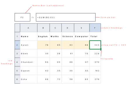
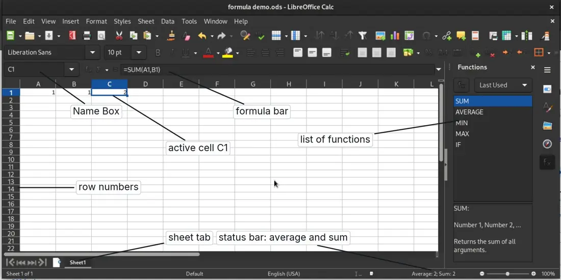
The formula bar shows what is really inside the active cell — a typed value or a formula — while the cell shows the result. The status bar at the bottom shows the Average, Count and Sum of the selected cells. The Excel ribbon has the tabs File, Home, Insert, Draw, Page Layout, Formulas, Data, Review, View, Automate and Help.
Counting the cells in a range
A range from column X to column Y and row m to row n has
(number of columns) × (number of rows) cells. Several separate ranges are
joined with a comma: A1:A5,C1:C5.
Problem. How many cells are in (a) B2:D6, (b) A1:E1, (c) C3:C12, (d) A1:B3,D1:D3? (e) Write the address of the cell in the 5th column and the 12th row.
Solution. (a) Columns B, C, D = 3; rows 2 to 6 = 5; cells = 3 × 5 = 15. (b) Columns A to E = 5; one row: 5. (c) One column; rows 3 to 12 = 12 − 3 + 1 = 10: 10. (d) A1:B3 has 2 × 3 = 6 cells and D1:D3 has 3, so 9. (e) The 5th column is E, so E12.
8.2 Entering and editing data; data types; AutoFill
Entering data. Click a cell (or move to it with the arrow keys), type, and press Enter (the next cell down becomes active) or Tab (the next cell to the right). Press Esc to cancel what you are typing.
Editing data. Click the cell and type again to replace its contents. To change part of it, double-click the cell or press F2 (or click in the formula bar), edit, and press Enter. Delete clears the contents of the selected cells; Ctrl + Z undoes.
Data types
| Type | What it is | Example | Lines up |
|---|---|---|---|
| Text (label) | letters, or numbers not used for calculation | Name, Kathmandu, Grade 8 | left |
| Number | values used in calculations | 85, 12.5, −40 | right |
| Currency, percentage | numbers with a format | Rs 1,200.00, 13% | right |
| Date and time | stored as numbers, so they can be subtracted | 24-10-2026, 10:30 | right |
| Formula | begins with =; shows its result |
=B2+C2 |
result's type |
| Logical (Boolean) | TRUE or FALSE, the answer of a comparison | =B2>=40 gives TRUE |
centre |
A number that should be kept as text, such as a roll number like 008, is
typed with an apostrophe in front: '008.
When something is wrong, the cell shows an error value:
| Error | Meaning | Fix |
|---|---|---|
##### |
the column is too narrow to show the number | widen the column |
#DIV/0! |
a number is divided by zero or by an empty cell | check the divisor |
#NAME? |
a misspelled function or name, e.g. =SUMM(A1:A5) |
correct the spelling |
#VALUE! |
text used where a number is needed | check the cells used |
#REF! |
the formula refers to a cell that was deleted | rewrite the reference |
AutoFill
The fill handle is the small square at the bottom-right corner of the active cell or selection. Dragging it copies the contents to the next cells or continues a series:
| Type in the first cell(s) | Drag the fill handle to get |
|---|---|
| 1, 2 (two cells selected) | 3, 4, 5, 6 … |
| 5, 10 | 15, 20, 25 … |
| Sunday | Monday, Tuesday, Wednesday … |
| Jan | Feb, Mar, Apr … |
| Grade 1 | Grade 2, Grade 3 … |
a formula =B2+C2 |
=B3+C3, =B4+C4 … (Section 8.3) |
| any other single value, e.g. 7 | 7, 7, 7 … (a copy) |
Double-clicking the fill handle fills a formula down as far as the data beside it goes. For more control: Home → Fill → Series (Calc: Sheet → Fill Cells → Fill Series).
8.3 Formulas and operators; relative and absolute cell references
A formula is an instruction that calculates a value. It always begins
with an equal sign (=) and may contain numbers, cell references,
operators and functions, e.g. =B2+C2+D2 or =F2/400*100.
Because a formula uses cell references instead of fixed numbers, it is recalculated automatically whenever any of those cells changes.
| Kind | Operator | Meaning | Example | Result |
|---|---|---|---|---|
| Arithmetic | + - |
add, subtract | =12+8-5 |
15 |
* / |
multiply, divide | =6*4/3 |
8 | |
^ |
power | =2^5 |
32 | |
% |
per cent | =200*13% |
26 | |
| Comparison | = <> |
equal, not equal | =5<>3 |
TRUE |
> < >= <= |
greater, less, at least, at most | =38>=40 |
FALSE | |
| Text | & |
join text | ="Ram "&"Thapa" |
Ram Thapa |
| Reference | : |
range | =SUM(A1:A5) |
— |
, |
union (several ranges) | =SUM(A1:A5,C1:C5) |
— |
Order of operations. As in mathematics (BODMAS): brackets first, then % and ^, then × and ÷ from left to right, then + and − from left to right.
Problem. Work out the result of each formula: (a) =2+3*4,
(b) =(2+3)*4, (c) =20-12/4, (d) =2^3*5. (e) Cells B2, C2, D2 and E2 hold
78, 85, 92 and 88. Write a formula for the average of the four marks and give
its result. (f) What is wrong with =B2+C2+D2+E2/4?
Solution. (a) Multiplication first: 3 × 4 = 12; 2 + 12 = 14.
(b) Brackets first: 5 × 4 = 20. (c) 12 ÷ 4 = 3; 20 − 3 = 17.
(d) 2³ = 8; 8 × 5 = 40.
(e) =(B2+C2+D2+E2)/4 = 343 ÷ 4 = 85.75.
(f) Only E2 is divided by 4, giving 78 + 85 + 92 + 22 = 277 — wrong. The
brackets are needed.
Relative and absolute references
When a formula is copied to another cell — with Copy and Paste or by dragging the fill handle — its references change.
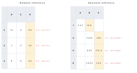
A relative reference such as B2 changes by the same number of rows and
columns as the formula moves when it is copied. An absolute reference such
as $B$1 has a dollar sign before the column letter and the row number and
does not change when the formula is copied. In a mixed reference
($B1 or B$1) only the part with the dollar sign is fixed.
Press F4 in Excel (Shift + F4 in Calc) while the cursor is in a reference
to cycle through B1 → $B$1 → B$1 → $B1.
Problem. A shop keeps the VAT rate 13% in cell B1. The prices of
four items are in B4:B7: 1200, 850, 2500 and 640 rupees. (a) Write a
formula for the VAT on the first item in C4 that can be copied down to C7, and
give the four results. (b) Write a formula in D4 for the price with VAT, copy
it down, and find the grand total in D8. (c) What goes wrong if C4 holds
=B4*B1 and is copied down?
Solution. (a) C4: =B4*$B$1. Copied down it becomes =B5*$B$1,
=B6*$B$1, =B7*$B$1. Results: 1200 × 13% = 156; 850 × 13% = 110.5;
2500 × 13% = 325; 640 × 13% = 83.2.
(b) D4: =B4+C4, copied down: 1356, 960.5, 2825, 723.2. D8:
=SUM(D4:D7) = 5864.7 rupees.
(c) With the relative B1, the copy in C5 becomes =B5*B2, C6 becomes
=B6*B3 and so on — pointing at empty cells, so the VAT shows 0. The $
signs keep every copy pointing at B1.
8.4 Functions: SUM, AVERAGE, MAX, MIN, COUNT and IF
A function is a ready-made formula with a name that does a particular
calculation. It is written =NAME(arguments), where the arguments — the
values or ranges it works on — are written in brackets and separated by commas.
| Function | What it returns | Example (B2:B6 hold 78, 55, 90, 42, 66) | Result |
|---|---|---|---|
SUM |
the total of the numbers | =SUM(B2:B6) |
331 |
AVERAGE |
the mean (sum ÷ how many numbers) | =AVERAGE(B2:B6) |
66.2 |
MAX |
the largest number | =MAX(B2:B6) |
90 |
MIN |
the smallest number | =MIN(B2:B6) |
42 |
COUNT |
how many cells contain numbers | =COUNT(B2:B6) |
5 |
IF |
one value if a condition is TRUE, another if FALSE | =IF(B2>=40,"Pass","Fail") |
Pass |
The AutoSum button (Σ) on the Home tab, or Alt + =, writes a SUM of the
numbers above or to the left for you; its arrow offers Average, Count Numbers,
Max and Min. (Calc: the Σ button beside the formula bar. In Calc the
separator between arguments may be a semicolon: =IF(B2>=40;"Pass";"Fail").)
The IF function has three arguments:
=IF(condition, value_if_true, value_if_false)
- the condition is a comparison that is TRUE or FALSE, e.g.
G2>=40; - text answers are written in double quotes:
"Pass"; - numbers and formulas need no quotes:
=IF(B2>1000,B2*5%,0)gives a 5% discount only on bills above Rs 1,000.
Problem. The mark sheet in Figure 1 has names in A2:A6 and marks out of 100 in English (B), Maths (C), Science (D) and Computer (E). (a) Write the formulas for the total in F2 and the percentage in G2, and give the results for all five students. (b) The school rule is that a student passes only with at least 40 in every subject. Write a formula for the result in H2. (c) Write formulas for the highest total, the lowest total, the class average of the totals and the number of students. (d) Bibek's Maths mark, 38, is corrected to 48. What changes?
Solution.
(a) F2: =SUM(B2:E2); G2: =F2/400*100. Fill both down to row 6.
| Name | English | Maths | Science | Computer | Total | % | Result |
|---|---|---|---|---|---|---|---|
| Aarati | 78 | 85 | 92 | 88 | 343 | 85.75 | Pass |
| Bibek | 55 | 38 | 61 | 70 | 224 | 56 | Fail |
| Chandani | 90 | 95 | 88 | 97 | 370 | 92.5 | Pass |
| Dipesh | 42 | 35 | 30 | 55 | 162 | 40.5 | Fail |
| Esha | 66 | 72 | 58 | 80 | 276 | 69 | Pass |
(b) H2: =IF(MIN(B2:E2)>=40,"Pass","Fail") — MIN finds the lowest mark; if even
that is 40 or more, every mark is. Bibek (38 in Maths) and Dipesh (30 and 35)
fail.
(c) =MAX(F2:F6) = 370; =MIN(F2:F6) = 162; =AVERAGE(F2:F6) = 1375 ÷ 5
= 275; =COUNT(F2:F6) = 5.
(d) Bibek's total becomes 234, his percentage 58.5 and his result Pass; the
class average becomes 277 — all recalculated automatically.
Forgetting the =: SUM(B2:E2) is stored as text and shows itself.
Using the wrong signs: multiply is * and divide is /, never × or ÷, and
a range uses a colon, B2:E2, not a dash. Testing the percentage
instead of every subject: =IF(G2>=40,"Pass","Fail") would pass Dipesh
(40.5%) although he failed three subjects. Read the rule, then choose the
formula.
COUNT counts only numbers. If D5 holds the word Absent instead of a mark,
=COUNT(D2:D6) gives 4, not 5, and AVERAGE divides by 4.
Nested IF. One IF can be placed inside another to choose among more than two
answers. For a grade: =IF(G2>=80,"A",IF(G2>=60,"B",IF(G2>=40,"C","D")))
gives A for Aarati (85.75) and Chandani (92.5), B for Esha (69), and C for
Bibek (56) and Dipesh (40.5).
8.5 Formatting cells; sorting and filtering data
Formatting cells
Formatting changes how cells look, not the values inside them. Select the cells, then use the Home tab or Format Cells (Ctrl + 1). (Calc: Format → Cells, also Ctrl + 1.)
| Group / dialog tab | What you can set |
|---|---|
| Font | font, size, bold, italic, colour |
| Alignment | left, centre, right; top, middle, bottom; Wrap Text; Merge & Center for a title across columns; text direction |
| Number | General, Number (decimal places), Currency (Rs), Percentage, Date; Increase/Decrease Decimal; thousands separator |
| Border and Fill | lines around cells; background colour |
| Cells → Format | column width, row height, AutoFit |
Conditional formatting colours cells automatically by their value: Home → Conditional Formatting → Highlight Cells Rules → Less Than… → type 40 → choose Light Red Fill shows every failing mark in red. (Calc: Format → Conditional → Condition.)
If a cell holds 85.756 and is formatted with one decimal place, it shows 85.8 but still holds 85.756, and formulas use 85.756. Likewise 0.13 formatted as a percentage shows 13% — so type 13% (or 0.13), not 13, in a cell that will be multiplied.
Sorting
Sorting arranges rows in ascending (A→Z, smallest first) or descending (Z→A, largest first) order of one column.
- Click any cell in the table (or select the whole table with its headings).
- Data → Sort. Tick My data has headers.
- Sort by: Total; Order: Largest to Smallest. Click Add Level to sort ties by a second column. Click OK.
The quick buttons Sort A to Z / Z to A (Calc: Data → Sort Ascending / Sort Descending) sort by the column of the active cell.
If only the Total column is selected and sorted, the totals move but the names do not, so every total is given to the wrong student. If Excel asks, choose Expand the selection.
Filtering
Filtering shows only the rows that meet a condition and hides the rest (nothing is deleted).
- Click inside the table. Data → Filter (Ctrl + Shift + L); a drop-down arrow appears in each heading. (Calc: Data → AutoFilter.)
- Click the arrow of a column, then tick the values you want, or choose Number Filters → Greater Than Or Equal To… and type a value.
- Row numbers of a filtered list turn blue; click the arrow → Clear Filter to show all rows again.
Problem. Using the mark sheet of Worked example 8.4: (a) list the students after sorting by Total, largest to smallest; (b) which students remain if the Maths column is filtered with Greater Than Or Equal To 60?
Solution. (a) Chandani 370, Aarati 343, Esha 276, Bibek 224, Dipesh 162. (b) Only rows with Maths ≥ 60 are shown: Aarati (85), Chandani (95) and Esha (72). Bibek (38) and Dipesh (35) are hidden, not deleted.
8.6 Charts: column, bar, line and pie
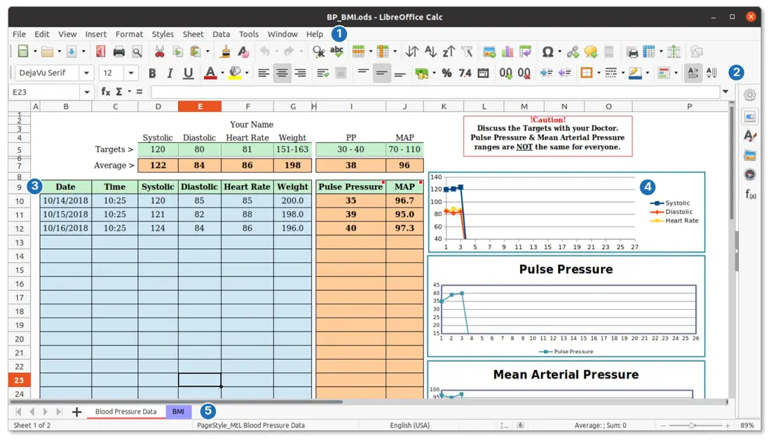
A chart (graph) is a picture of worksheet data that makes comparisons and trends easy to see. It is linked to its data: change a number and the chart redraws itself.
Parts of a chart: chart title; axes (the horizontal category axis and the vertical value axis) with axis titles; data series (the bars, line or slices); data labels (the numbers on them); legend (which colour means what); gridlines; and the plot area.
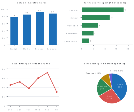
| Chart | Looks like | Best for | Example |
|---|---|---|---|
| Column | vertical bars | comparing separate items or groups | marks in each subject; sales of each shop |
| Bar | horizontal bars | comparing items, especially with long names | votes for each sport or candidate |
| Line | points joined by a line | change over time (a trend) | temperature through a week; monthly savings |
| Pie | a circle cut into slices | parts of one whole, as percentages | how a family's income is spent |
Inserting a chart in Excel
- Select the data with its labels, e.g. A1:B6 (subjects in A, marks in B).
- Insert → Recommended Charts, or choose a type in the Charts group: Insert Column or Bar Chart, Insert Line, Insert Pie.
- With the chart selected, the Chart Design tab offers Add Chart Element (Chart Title, Axis Titles, Data Labels, Legend), Chart Styles, Switch Row/Column, Change Chart Type and Move Chart (to its own sheet). The + button beside the chart turns elements on and off.
- Click the title on the chart and type a meaningful one.
(Calc: select the data → Insert → Chart → the Chart Wizard asks for the chart type, data range, data series and chart elements → Finish.)
Problem. A family spends Rs 12,000 on food, Rs 8,000 on rent, Rs 6,000 on education, Rs 3,000 on transport and Rs 1,000 on other things in a month. (a) Which chart shows how the money is shared out? (b) Work out the percentage and the angle of each slice, as the spreadsheet does. (c) Write the formulas if the amounts are in B2:B6.
Solution. (a) A pie chart: the data are parts of one whole.
(b) Total = 12,000 + 8,000 + 6,000 + 3,000 + 1,000 = Rs 30,000.
Food: 12,000 ÷ 30,000 = 40%, angle 0.40 × 360° = 144°.
Rent: 8,000 ÷ 30,000 ≈ 26.7%, angle 96°.
Education: 20%, angle 72°. Transport: 10%, angle 36°.
Others: ≈ 3.3%, angle 12°. Check: 144 + 96 + 72 + 36 + 12 = 360°.
(c) B7: =SUM(B2:B6); C2: =B2/$B$7 formatted as Percentage, filled down;
D2: =B2/$B$7*360, filled down. The $ keeps every row dividing by the total.
In the lab, build the mark sheet of Worked example 8.4 for ten classmates
(use your own unit-test marks with their permission, or invented ones). Use
AutoFill for the roll numbers, SUM, percentage, MAX, MIN, AVERAGE and COUNT, an
IF for the result and a nested IF for the grade. Format it with a merged,
centred title, borders and conditional formatting for marks below 40. Sort it by
total, filter the students above 60% in Computer, and make a column chart of
your own marks. Save it as Marksheet.xlsx.
Write the formula exactly as typed — =AVERAGE(B2:E2) — and then the
result with a line of working: (78 + 85 + 92 + 88) ÷ 4 = 85.75. When a
formula is copied, write the new formula in the new cell, e.g. "=B4*$B$1 in C4
becomes =B5*$B$1 in C5".
Chapter summary
- A spreadsheet (Excel, Calc, Google Sheets) calculates with data in rows and columns. A workbook (.xlsx, .ods) holds worksheets; a cell is where a row (number) meets a column (letter); its address is like C5; a range is written B2:E6 and has columns × rows cells.
- Data types: text (left), numbers (right), currency, percentage, dates,
formulas, TRUE/FALSE. Errors:
#####,#DIV/0!,#NAME?,#VALUE!,#REF!. AutoFill with the fill handle copies or continues series. - Formulas start with =; operators
+ - * / ^ %, comparisons= <> > < >= <=,&; brackets first, then ^, then × ÷, then + −. - Relative references (B2) change when copied; absolute (
$B$1) do not; mixed$B1,B$1; F4 toggles. - Functions:
SUM,AVERAGE,MAX,MIN,COUNT(numbers only),IF(condition, if_true, if_false); nested IF for grades. - Formatting (Ctrl + 1) changes appearance, not values; sort the whole table (Data → Sort); filter hides rows (Data → Filter).
- Charts: column and bar compare items, line shows change over time, pie shows parts of a whole (angle = share × 360°).
Practice questions
Group A — Objective (1 mark each)
- A spreadsheet file is called a [1]aworksheetbworkbookccelldrange
- The address of the cell in column D and row 7 is [1]a7DbD7cD:7d4,7
- How many cells are in the range B3:D7? [1]a10b12c15d21
- Every formula must begin with [1]a
+b#c=d$ - The result of
=10+6/2is [1]a8b13c16d3 - Which is an absolute cell reference? [1]a
B5b$B5cB$5d$B$5 - If B2:B5 hold 10, 20, "Absent" and 30, then
=COUNT(B2:B5)gives [1]a4b3c60d20 =IF(C2>=40,"Pass","Fail")when C2 holds 38 gives [1]aPassbFailc38dTRUE- The small square at the bottom-right corner of the active cell is the [1]aName Boxbfill handlecformula bardsheet tab
- A cell shows
#####. This means [1]athe formula is wrongbthe column is too narrowcthe value is negativedthe file is damaged - Which chart is best for showing how a whole is divided into parts? [1]alinebcolumncpiedbar
- The formula
=A2*B1in C2 is copied to C3. It becomes [1]a=A2B1b=A3B2c=A3B1d=B3C2
Answers to Group A
1. (b) — a workbook holds worksheets.
2. (b) — column letter, then row number.
3. (c) — 3 columns (B, C, D) × 5 rows (3 to 7) = 15.
4. (c) — the equal sign.
5. (b) — 6 ÷ 2 = 3 first, then 10 + 3 = 13.
6. (d) — dollar signs before both the column and the row.
7. (b) — COUNT counts only the three numbers.
8. (b) — 38 is not ≥ 40, so the FALSE value is shown.
9. (b) — the fill handle, used for AutoFill.
10. (b) — widen the column to see the number.
11. (c) — a pie chart shows parts of a whole.
12. (b) — both relative references move down one row.
Group B — Short answer (2 marks each)
- Define cell, cell address and range with an example of each. [2]
- Differentiate between a workbook and a worksheet. [2]
- Differentiate between a formula and a function, with an example of each. [2]
- What is AutoFill? Write what appears when "Monday" is filled down three cells. [2]
- Differentiate between relative and absolute cell references. [2]
- Cells A1:A4 hold 12, 18, 25 and 5. Write the result of
=SUM(A1:A4),=AVERAGE(A1:A4),=MAX(A1:A4)and=MIN(A1:A4). [2] - Write an IF function that shows "Eligible" if the age in B2 is 16 or more and "Not eligible" otherwise. [2]
- Differentiate between sorting and filtering. [2]
- Write any four parts of a chart. [2]
- Which chart would you use to show(a) the monthly temperature of Pokhara over a year,(b) the share of votes won by four candidates? Give reasons. [2]
Answers to Group B
1. A cell is the box where a row and a column meet, e.g. the cell holding Aarati's Maths mark. A cell address is its column letter and row number, e.g. C2. A range is a rectangular block of cells written first:last, e.g. B2:E6.
2. A workbook is the whole spreadsheet file (e.g. Marks.xlsx); a worksheet
is one grid of rows and columns inside it, chosen by a sheet tab. One workbook
can hold many worksheets.
3. A formula is any calculation the user writes, beginning with =, e.g.
=B2+C2+D2. A function is a built-in, named formula, e.g. =SUM(B2:D2).
Functions can be used inside formulas.
4. AutoFill copies cell contents or continues a series when the fill handle is dragged. Filling "Monday" down three cells gives Tuesday, Wednesday, Thursday.
5. A relative reference (B2) changes when the formula is copied, by the
number of rows and columns moved. An absolute reference ($B$2) stays fixed on
the same cell when copied, e.g. a VAT rate in one cell.
6. SUM = 12 + 18 + 25 + 5 = 60; AVERAGE = 60 ÷ 4 = 15; MAX = 25; MIN = 5.
7. =IF(B2>=16,"Eligible","Not eligible").
8. Sorting rearranges all the rows in ascending or descending order of a column; filtering shows only the rows that meet a condition and hides the others without changing their order.
9. Any four: chart title, axes, axis titles, data series (bars, line or slices), data labels, legend, gridlines, plot area.
10. (a) A line chart, because temperature changes over time and a line shows the trend. (b) A pie chart, because the votes are parts of one whole (total votes).
Group C — Long answer (4 marks each)
- Explain any four functions of a spreadsheet with syntax and an example of each. [4]
- In a sheet, B2:B6 hold the prices 450, 1200, 880, 2300 and 170 and the discount rate 10% is in E1.(a) Write a formula in C2 for the discount that can be copied down, and give all five results.(b) Write a formula for the price after discount in D2, and find the total of D2:D6. [2+2]
- Write the steps to(a) sort a mark sheet by total, largest first, and(b) show only the students who scored at least 60 in Science. [2+2]
- Describe the column, line and pie charts with one use of each, and write the steps to insert a column chart. [3+1]
- The marks of a student out of 100 are 64, 38, 75, 81 and 57 in B2:F2. Write formulas for the total, the percentage (out of 500), the highest and lowest marks, and a result that is "Pass" only if every mark is at least 40. Give each result. [4]
Answers to Group C
1. Any four. SUM(range) adds numbers: =SUM(B2:B6) gives 331 for 78,
55, 90, 42, 66. AVERAGE(range) gives the mean: =AVERAGE(B2:B6) = 66.2.
MAX(range) gives the largest: =MAX(B2:B6) = 90. MIN(range) gives the
smallest: =MIN(B2:B6) = 42. COUNT(range) counts cells with numbers:
=COUNT(B2:B6) = 5. IF(condition, value_if_true, value_if_false):
=IF(B2>=40,"Pass","Fail") gives Pass for 78.
2. (a) C2: =B2*$E$1 (E1 must be absolute), filled down. Results: 450 ×
10% = 45; 1200 → 120; 880 → 88; 2300 → 230; 170 → 17.
(b) D2: =B2-C2, filled down: 405, 1080, 792, 2070, 153. Total
=SUM(D2:D6) = 4500.
3. (a) Click any cell in the table → Data → Sort → tick My data has headers → Sort by Total → Order Largest to Smallest → OK. (b) Click in the table → Data → Filter → click the arrow on the Science heading → Number Filters → Greater Than Or Equal To → type 60 → OK. Only those students' rows are shown; Clear Filter shows all again.
4. Column chart: vertical bars comparing separate items — marks in each subject. Line chart: points joined by a line showing change over time — temperature through a week. Pie chart: a circle divided into slices showing parts of a whole — a family's spending. Steps for a column chart: select the data with labels → Insert → Insert Column or Bar Chart → 2-D Clustered Column → add a chart title with Chart Design → Add Chart Element → Chart Title.
5. Total: =SUM(B2:F2) = 64 + 38 + 75 + 81 + 57 = 315. Percentage:
=SUM(B2:F2)/500*100 (or the total's cell /500100) = 63. Highest:
=MAX(B2:F2) = 81. Lowest: =MIN(B2:F2) = 38. Result:
=IF(MIN(B2:F2)>=40,"Pass","Fail") gives Fail*, because the lowest mark,
38, is below 40.
Practise more: Computer Science question bank