Unit 20 · Electricity and Magnetism · 3 teaching hours · 21 min read
Electric field
What the syllabus asks for 3
- Electric field due to point charges; Field lines
- Gauss Law: Electric Flux
- Application of Gauss law: field of a charged sphere, line charge, charged plane conductor
Coulomb's law tells you the force one charge exerts on another, but it says nothing about how the push gets across empty space. The modern answer is the field: a charge alters the space around it, and any second charge placed in that space responds to the local condition it finds there. This unit builds the field of a point charge, draws it, and then introduces Gauss's law — a shortcut that reduces a page of integration to three lines whenever the charge distribution is symmetric.
Group B nearly always wants one Gauss-law derivation (sphere, line, or plane) and one numerical on the combined field of two point charges. Learn the three derivations as one family: they differ only in the Gaussian surface you choose.
20.1 Electric field due to point charges; Field lines
Place a small positive test charge q_0 at a point and measure the force \vec{F} on it. The electric field intensity at that point is
The electric field intensity at a point is the force experienced per unit positive charge placed at that point. It is a vector, directed along the force on a positive charge, with SI unit newton per coulomb (N C⁻¹), equivalently volt per metre (V m⁻¹).
The limit q_0 \to 0 matters: a large test charge would itself push the source charges around and change the very field we are trying to measure.
For a point charge Q, Coulomb's law gives F = \dfrac{1}{4\pi\varepsilon_0} \dfrac{Qq_0}{r^{2}}, so dividing by q_0,
with k = 1/4\pi\varepsilon_0 = 9.0\times10^{9}\ \text{N m}^{2}\text{C}^{-2} and \varepsilon_0 = 8.85\times10^{-12}\ \text{C}^{2}\text{N}^{-1}\text{m}^{-2}. The field points away from a positive charge and towards a negative one.
Because forces add as vectors, so do fields. This is the principle of superposition: the field of a group of charges is the vector sum of the fields each would produce alone,
Electric field lines
A field line is a curve drawn so that the tangent at every point gives the direction of \vec{E} there. Faraday invented them to make an invisible field visible, and their rules are examined directly.
- They start on positive charge and end on negative charge (or run to infinity).
- The tangent at any point gives the direction of the field at that point.
- They never cross. If two lines crossed, the field would have two directions at one point, which is impossible.
- Where the lines crowd together the field is strong; where they spread out it is weak. The number of lines per unit cross-sectional area measures E.
- They are always perpendicular to the surface of a conductor in equilibrium, and there are no lines inside a conductor — the field there is zero.
- They do not form closed loops in electrostatics, and they are continuous curves with no breaks in charge-free space.
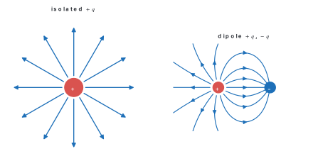
A charge released from rest does follow the line at first, but a charge with sideways velocity does not travel along a field line. The line gives the direction of the force, not of the motion.
Problem. Point charges q_1 = +9\ \mu\text{C} and q_2 = -4\ \mu\text{C} are held 1\ \text{m} apart. Find the point on the line joining them where the resultant field is zero.
Solution. Between the charges both fields point from q_1 towards q_2, so they add and cannot cancel. Outside, on the side of the larger charge, the field of q_1 always dominates because it is both bigger and nearer. So the null point lies beyond the smaller charge q_2.
Let it be a distance d beyond q_2, i.e. (1+d) from q_1. Then
Cross-multiplying, 3d = 2 + 2d, so d = 2\ \text{m}. The field vanishes 2\ \text{m} beyond the -4\ \mu\text{C} charge, i.e. 3\ \text{m} from the +9\ \mu\text{C} charge on the far side.
Problem. Two equal charges q = +2\ \mu\text{C} sit at A(-3\ \text{cm}, 0) and B(+3\ \text{cm}, 0). Find the field at P(0, 4\ \text{cm}).
Solution. AP = BP = \sqrt{3^{2}+4^{2}} = 5\ \text{cm} = 0.05\ \text{m}. Each charge gives
By symmetry the horizontal components are equal and opposite and cancel. The vertical components each carry a factor \cos\theta = 4/5 = 0.8, so
directed along +y, i.e. straight away from AB.
20.2 Gauss Law: Electric Flux
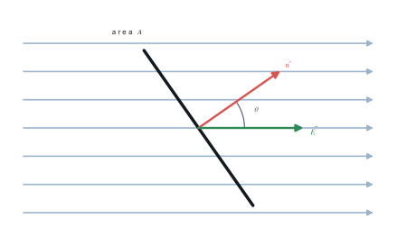
Electric flux measures how much field "flows" through a surface. For a flat area A in a uniform field \vec{E}, with \theta the angle between \vec{E} and the outward normal to the area,
Flux is a scalar, with SI unit N m² C⁻¹ (equivalently V m). It is maximum (EA) when the surface faces the field squarely, and zero when the surface lies edge-on, \theta = 90^{\circ}. For a curved surface in a non-uniform field we chop it into elements d\vec{A} and add:
The net electric flux through any closed surface is 1/\varepsilon_0 times the total charge enclosed by that surface:
The imaginary closed surface used is called a Gaussian surface.
We start from Coulomb's law and reach Gauss's law, by computing the total flux out of a sphere drawn around a single charge.
Setting up. Put a charge q at the centre of an imaginary sphere of radius r. The sphere is chosen with the charge at the centre because that is the shape the field respects.
Step 1 — the field on the sphere. By Coulomb's law, at every point of the sphere
and this has the same value everywhere on the sphere, because every point is the same distance r away.
Step 2 — the direction of the field. The field of a point charge is radial, and the outward normal d\vec{A} of a sphere is also radial. So the angle between them is zero everywhere:
Step 3 — write the flux integral:
Step 4 — put \cos\theta = 1 and take the constant E outside the integral. We may do this because Step 1 showed E has the same value at every point:
Step 5 — do the remaining integral. \oint dA is just the total surface area of the sphere:
Step 6 — substitute Steps 1 and 5:
Step 7 — cancel 4\pi r^{2}, which appears on top and bottom:
Result.
What it means. r disappeared in Step 7, so the flux is the same through a big sphere as through a small one. Physically, the field weakens as 1/r^{2} but the area grows as r^{2}, and the two effects cancel exactly. Since the same field lines cross every closed surface drawn round the charge, the result holds for a surface of any shape, not just a sphere — which is what makes Gauss's law useful.
Conditions used. The medium is vacuum or air (otherwise \varepsilon_0 becomes \varepsilon); the charge is a point charge at the centre; and the surface is closed.
Two consequences are worth stating separately. First, only the charge inside the surface counts: a charge outside contributes equal inward and outward flux, netting zero. Second, if q_{enc} = 0 the net flux is zero — but that does not mean E = 0 everywhere on the surface.
Problem. A point charge of 8.85\ \mu\text{C} is placed at the centre of a cube of side 20\ \text{cm}. Find (a) the total flux through the cube and (b) the flux through one face.
Solution.
(a) \Phi = \dfrac{q}{\varepsilon_0} = \dfrac{8.85\times10^{-6}}{8.85\times10^{-12}} = 1.0\times10^{6}\ \text{N m}^{2}\text{C}^{-1}.
(b) By symmetry the six faces share the flux equally:
The side of the cube never entered the calculation — flux depends only on the charge enclosed.
20.3 Application of Gauss law: field of a charged sphere, line charge, charged plane conductor
The method is always the same three steps: (i) identify the symmetry, (ii) choose a Gaussian surface on which E is constant and either parallel or perpendicular to d\vec{A}, (iii) equate EA to q_{enc}/\varepsilon_0.
(a) Uniformly charged conducting sphere
Let a conducting sphere of radius R carry charge Q, which spreads uniformly over its outer surface.
We start from Gauss's law and reach the field at three places: outside the sphere, at its surface, and inside it.
Setting up. A conducting sphere of radius R carries charge Q. Because it is a conductor, all the charge sits on the outer surface, spread evenly. The surface charge density is \sigma = Q/(4\pi R^{2}).
Case 1 — outside, r > R.
Step 1 — choose the Gaussian surface. Take a sphere of radius r concentric with the charged sphere. The charge distribution is spherically symmetric, so the field must be radial and must have the same magnitude everywhere on this surface.
Step 2 — write the flux. Field parallel to the outward normal, constant magnitude, total area 4\pi r^{2}:
Step 3 — find the enclosed charge. The Gaussian sphere is bigger than the conductor, so it contains all of it:
Step 4 — apply Gauss's law, \Phi = q_{enc}/\varepsilon_0:
Step 5 — divide both sides by 4\pi r^{2}:
So outside, the sphere behaves exactly like a point charge Q at its centre.
Case 2 — at the surface, r = R.
Step 6 — put r = R in the result of Step 5:
Step 7 — rewrite using the surface charge density. From \sigma = Q/(4\pi R^{2}) we get Q = 4\pi R^{2}\sigma. Substituting:
This is the largest value the field reaches anywhere.
Case 3 — inside, r < R.
Step 8 — choose a Gaussian sphere of radius r inside the metal. Its flux expression is the same as before:
Step 9 — find the enclosed charge. All the charge lies on the outer surface, at radius R, which is outside this Gaussian sphere. So it encloses nothing:
Step 10 — apply Gauss's law:
Step 11 — divide by 4\pi r^{2}, which is not zero:
Result.
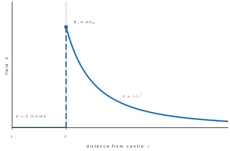
What it means. The field is zero everywhere inside a charged conductor, jumps suddenly to \sigma/\varepsilon_0 at the surface, then dies away as 1/r^{2}. The zero inside is the principle of electrostatic shielding — why you are safe inside a car in a thunderstorm, and why sensitive instruments are put in metal boxes.
Conditions used. The sphere is a conductor in electrostatic equilibrium (so all charge is on the outer surface and E = 0 within the metal), the charge is spread uniformly, and the surrounding medium is air.
(b) Infinitely long straight line charge
Let charge be spread along a long straight wire with linear charge density \lambda (charge per metre).
We start from Gauss's law with a cylindrical surface and reach the field at distance r from a long charged wire.
Setting up. Charge is spread along a long straight wire with linear charge density \lambda (coulombs per metre). We want E at perpendicular distance r from the wire.
Step 1 — use the symmetry to guess the field's direction. The wire looks the same from every direction around it and the same from every point along it, so the field can only point straight out from the wire (radially), and its magnitude can depend only on r.
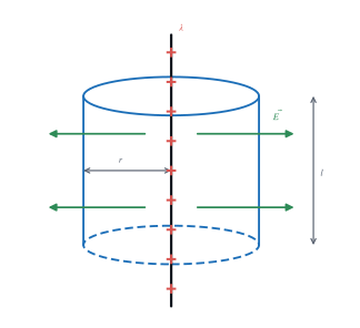
Step 2 — choose the Gaussian surface to match that symmetry. Take a cylinder of radius r and length l, with the wire along its axis.
Step 3 — flux through the two flat ends. There the outward normal points along the wire, while \vec{E} points perpendicular to the wire. Perpendicular vectors give no flux:
Step 4 — flux through the curved surface. Here \vec{E} is parallel to the outward normal everywhere, and has the same magnitude everywhere (Step 1). The curved area is 2\pi r l:
Step 5 — total flux is the sum of Steps 3 and 4:
Step 6 — find the enclosed charge. A length l of wire lies inside the cylinder, and each metre carries \lambda:
Step 7 — apply Gauss's law:
Step 8 — cancel l from both sides. The length of cylinder we chose was arbitrary, so it had better not appear in the answer — and it does not:
Step 9 — divide both sides by 2\pi r:
Step 10 — write it with k = 1/(4\pi\varepsilon_0). Since \dfrac{1}{2\pi\varepsilon_0} = \dfrac{2}{4\pi\varepsilon_0} = 2k:
Result.
What it means. The field falls off as 1/r, not as 1/r^{2}. A line of charge is a "fatter" source than a point charge: as you move away, the wire still stretches out beside you, so the field dies more slowly. It is directed away from the wire if \lambda is positive, towards it if negative.
Conditions used. The wire must be effectively infinite — in practice, r much smaller than the length of the wire, and the point not near either end. Otherwise Step 1's symmetry fails.
Note the field falls off as 1/r, not 1/r^{2} — a line of charge is a "fatter" source than a point.
(c) Charged plane conductor
We start from Gauss's law with a flat "pill box" and reach the field close to a large charged plate — and then see why a non-conducting sheet gives half as much.
Setting up. A large flat conductor carries surface charge density \sigma (coulombs per square metre). We want E at a point just outside its surface. Because the plate is large and flat, the field there must be perpendicular to the surface and the same at all nearby points.
Step 1 — choose the Gaussian surface. Take a short cylinder (a "pill box") of cross-sectional area A, with one flat face just outside the surface and the other buried inside the metal.
Step 2 — flux through the inner face is zero. Inside a conductor in equilibrium E = 0, so nothing crosses that face:
Step 3 — flux through the curved side is zero. There \vec{E} lies along the surface, parallel to the curved wall, so it crosses nothing:
Step 4 — flux through the outer face. Here \vec{E} is perpendicular to the face, i.e. parallel to its outward normal, and constant across it:
Step 5 — total flux is the sum of Steps 2, 3 and 4:
Step 6 — find the enclosed charge. The pill box cuts out a patch of surface of area A, and each square metre carries \sigma:
Step 7 — apply Gauss's law:
Step 8 — cancel A from both sides:
Now the thin non-conducting sheet.
Step 9 — what changes. A thin insulating sheet has charge on it but no interior in which E must vanish. The field now comes out of both faces of the pill box, so the flux is doubled:
Step 10 — the enclosed charge is the same \sigma A, so Gauss's law gives
Step 11 — cancel A and divide by 2:
Result.
What it means. r never appeared, so the field near a large plate does not weaken as you move away — it is uniform. That is exactly why a parallel-plate capacitor has a uniform field between its plates. The factor of two is not a formula to memorise but a consequence of how many faces the flux comes out of.
Conditions used. The plate is large compared with the distance of the point from it (so edge effects can be ignored), and the charge is spread uniformly.
Use \sigma/\varepsilon_0 just outside a charged conductor (all the charge is on one face and there is no field inside the metal). Use \sigma/2\varepsilon_0 for a thin non-conducting sheet, which radiates field from both sides. Mixing them up is the single most common Group B error in this unit.
| Charge distribution | Gaussian surface | Field | Dependence |
|---|---|---|---|
| Point charge q | sphere | \dfrac{kq}{r^{2}} | 1/r^{2} |
| Conducting sphere, r>R | sphere | \dfrac{kQ}{r^{2}} | 1/r^{2} |
| Conducting sphere, r<R | sphere | 0 | — |
| Long line charge | cylinder | \dfrac{\lambda}{2\pi\varepsilon_0 r} | 1/r |
| Charged conductor surface | pill box | \dfrac{\sigma}{\varepsilon_0} | independent of r |
| Thin non-conducting sheet | pill box | \dfrac{\sigma}{2\varepsilon_0} | independent of r |
Problem. A hollow metal sphere of radius 10\ \text{cm} carries a charge of 5\ \mu\text{C}. Find the field at r = 5\ \text{cm}, at the surface, and at r = 20\ \text{cm} from the centre. Also find the surface charge density.
Solution.
At r = 5\ \text{cm} (inside the conductor): E = 0.
At the surface, r = R = 0.10\ \text{m}:
At r = 0.20\ \text{m}:
Surface charge density: \sigma = \dfrac{Q}{4\pi R^{2}} = \dfrac{5\times10^{-6}}{4\pi(0.10)^{2}} = 3.98\times10^{-5}\ \text{C m}^{-2}.
As a check, \sigma/\varepsilon_0 = 3.98\times10^{-5}/8.85\times10^{-12} = 4.5\times10^{6}\ \text{N C}^{-1}, matching the surface field.
Chapter summary
- \vec{E} = \vec{F}/q_0, measured in N C⁻¹ = V m⁻¹; for a point charge E = kQ/r^{2} with k = 1/4\pi\varepsilon_0 = 9\times10^{9} SI units.
- Fields superpose vectorially: \vec{E} = \sum \vec{E}_i.
- Field lines run from + to -, never cross, are densest where E is largest, meet conductors at right angles and do not exist inside a conductor.
- Electric flux \Phi_E = EA\cos\theta, a scalar with unit N m² C⁻¹.
- Gauss's law: \oint \vec{E}\cdot d\vec{A} = q_{enc}/\varepsilon_0; only enclosed charge contributes.
- Charged conducting sphere: E = kQ/r^{2} outside, \sigma/\varepsilon_0 at the surface, 0 inside.
- Long line charge: E = \lambda/2\pi\varepsilon_0 r (falls as 1/r).
- Charged conductor surface: E = \sigma/\varepsilon_0; thin non-conducting sheet: E = \sigma/2\varepsilon_0. Both are uniform.
Practice questions
Group A — Multiple choice (1 mark each)
- The SI unit of electric field intensity is [1]aN CbN C⁻¹cC N⁻¹dN m² C⁻¹
- The electric field at a point inside a charged hollow metal sphere is [1]akQ/r^{2}b\sigma/\varepsilon_0czerodinfinite
- The net electric flux through a closed surface enclosing an electric dipole is [1]aq/\varepsilon_0b2q/\varepsilon_0czerodq/2\varepsilon_0
- For an infinitely long charged straight wire, E varies with distance r as [1]a1/r^{2}b1/rcrdindependent of r
- Two electric field lines can never intersect because [1]athey are parallelbthe field would have two directions at one pointccharge is quantiseddflux would be infinite
Answers to Group A
1. (b) — E = F/q, so newton per coulomb.
2. (c) — the Gaussian surface inside encloses no charge.
3. (c) — q_{enc} = +q - q = 0.
4. (b) — the cylindrical Gaussian surface gives E = \lambda/2\pi\varepsilon_0 r.
5. (b) — a unique tangent means a unique field direction.
Group B — Short answer (5 marks each)
- Define electric field intensity and electric flux. State Gauss's law and name its SI units. [5]
- Using Gauss's law, derive an expression for the electric field due to an infinitely long straight uniformly charged wire. [5]
- Two point charges +9\ \mu\text{C} and -4\ \mu\text{C} are placed 1\ \text{m} apart in air. Locate the point where the resultant electric field is zero. [5]
- A charge of 17.7\ \mu\text{C} is placed at the centre of a cube of side 10\ \text{cm}. Calculate the electric flux through one face of the cube. [5]
- A metal sphere of radius 5\ \text{cm} carries a charge of 2\ \mu\text{C}. Find the field at 2\ \text{cm}, at 5\ \text{cm} and at 10\ \text{cm} from its centre. [5]
Answers to Group B
3. The point lies beyond the -4\ \mu\text{C} charge. With d measured from it, 9/(1+d)^{2} = 4/d^{2} gives 3d = 2+2d, so d = 2\ \text{m} — that is, 3\ \text{m} from the +9\ \mu\text{C} charge on the side away from it.
4. Total flux = q/\varepsilon_0 = 17.7\times10^{-6}/8.85\times10^{-12} = 2.0\times10^{6}\ \text{N m}^{2}\text{C}^{-1}. One face gets one sixth: 3.33\times10^{5}\ \text{N m}^{2}\text{C}^{-1}. The side length is irrelevant.
5. At 2\ \text{cm} (inside): E = 0. At the surface: E = 9\times10^{9}\times2\times10^{-6}/(0.05)^{2} = 7.2\times10^{6}\ \text{N C}^{-1}. At 10\ \text{cm}: E = 9\times10^{9}\times2\times10^{-6}/(0.10)^{2} = 1.8\times10^{6}\ \text{N C}^{-1}.
Group C — Long answer (8 marks each)
- (a) State Gauss's law and prove it for a point charge enclosed by a spherical surface. [3](b) Using it, obtain the electric field due to a uniformly charged conducting sphere at a point outside, on and inside the sphere, and sketch E against r. [5]
- (a) Apply Gauss's law to find the electric field near the surface of a charged plane conductor, and explain why a thin non-conducting sheet of the same charge density gives half that value. [4](b) Two large parallel metal plates carry surface charge densities +3.54\times10^{-6}\ \text{C m}^{-2} and -3.54\times10^{-6}\ \text{C m}^{-2}. Find the field between the plates and the force on an electron placed there. [4]
Answers to Group C
1. (a) Put q at the centre of a sphere of radius r. E = kq/r^{2} is constant and parallel to d\vec{A}, so \oint \vec{E}\cdot d\vec{A} = E(4\pi r^{2}) = q/\varepsilon_0. (b) Outside, E = kQ/r^{2}; at the surface, E = kQ/R^{2} = \sigma/\varepsilon_0; inside, the enclosed charge is zero so E = 0. The graph is flat at zero up to R, jumps to \sigma/\varepsilon_0, then decays as 1/r^{2}.
2. (b) Between the plates, E = \sigma/\varepsilon_0 = 3.54\times10^{-6}/8.85\times10^{-12} = 4.0\times10^{5}\ \text{V m}^{-1}, directed from the positive to the negative plate. Force on an electron: F = eE = 1.6\times10^{-19}\times4.0\times10^{5} = 6.4\times10^{-14}\ \text{N}, directed towards the positive plate.
Practise more: Physics question bank